

6.2 NLSE: Nonlinear Least-Squares Parameter Estimation
147
∇∇∇r(x) =
1
r(x)
∂
∂x j
f 1
∂f 1
∂x i
+ · · · + f 2M
∂f 2M
∂x i
, i,j = 1, . . . , N
=
1
r(x)
α
∂f α
∂x j
∂f α
∂x i
+ f α
∂ 2 f α
∂x j ∂x i
, α = 1, . . . , 2M . (6.10)
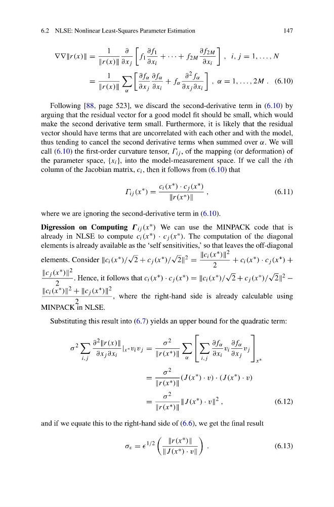
Following [88, page 523], we discard the second-derivative term in (6.10) by
arguing that the residual vector for a good model fit should be small, which would
make the second derivative term small. Furthermore, it is likely that the residual
vector should have terms that are uncorrelated with each other and with the model,
thus tending to cancel the second derivative terms when summed over α. We will
call (6.10) the first-order curvature tensor, Γ ij , of the mapping (or deformation) of
the parameter space, {x i }, into the model-measurement space. If we call the ith
column of the Jacobian matrix, c i , then it follows from (6.10) that
Γ ij (x
∗ ) =
c i (x ∗ ) · c j (x ∗ )
r(x ∗ )
,
(6.11)
where we are ignoring the second-derivative term in (6.10).
Digression on Computing Γ ij (x ∗ ) We can use the MINPACK code that is
already in NLSE to compute c i (x ∗ ) · c j (x ∗ ). The computation of the diagonal
elements is already available as the ‘self sensitivities,’ so that leaves the off-diagonal
elements. Consider c i (x ∗ )/
√
2 + c j (x ∗ )/
√
2 2 =
c i (x ∗ ) 2
2
+ c i (x ∗ ) · c j (x ∗ ) +
c j (x ∗ ) 2
2
. Hence, it follows that c i (x ∗ ) · c j (x ∗ ) = =c i (x ∗ )/
√
2 + c j (x ∗ )/
√
2 2 −
c i (x ∗ ) 2 + +c j (x ∗ ) 2
2
, where the right-hand side is already calculable using
MINPACK in NLSE.
Substituting this result into (6.7) yields an upper bound for the quadratic term:
σ
2
i,j
∂ 2 r(x)
∂x j ∂x i
| x ∗ v i v j =
σ 2
r(x ∗ )
α
⎡
⎣
i,j
∂f α
∂x i
v i
∂f α
∂x j
v j
⎤
⎦
x ∗
=
σ 2
r(x ∗ )
(J (x
∗ ) · v) · (J (x
∗ ) · v)
=
σ 2
r(x ∗ )
J (x
∗ ) · v
2 ,
(6.12)
and if we equate this to the right-hand side of (6.6), we get the final result
σ v =
1/2
r(x ∗ )
J (x ∗ ) · v
.
(6.13)
147
∇∇∇r(x) =
1
r(x)
∂
∂x j
f 1
∂f 1
∂x i
+ · · · + f 2M
∂f 2M
∂x i
, i,j = 1, . . . , N
=
1
r(x)
α
∂f α
∂x j
∂f α
∂x i
+ f α
∂ 2 f α
∂x j ∂x i
, α = 1, . . . , 2M . (6.10)
Following [88, page 523], we discard the second-derivative term in (6.10) by
arguing that the residual vector for a good model fit should be small, which would
make the second derivative term small. Furthermore, it is likely that the residual
vector should have terms that are uncorrelated with each other and with the model,
thus tending to cancel the second derivative terms when summed over α. We will
call (6.10) the first-order curvature tensor, Γ ij , of the mapping (or deformation) of
the parameter space, {x i }, into the model-measurement space. If we call the ith
column of the Jacobian matrix, c i , then it follows from (6.10) that
Γ ij (x
∗ ) =
c i (x ∗ ) · c j (x ∗ )
r(x ∗ )
,
(6.11)
where we are ignoring the second-derivative term in (6.10).
Digression on Computing Γ ij (x ∗ ) We can use the MINPACK code that is
already in NLSE to compute c i (x ∗ ) · c j (x ∗ ). The computation of the diagonal
elements is already available as the ‘self sensitivities,’ so that leaves the off-diagonal
elements. Consider c i (x ∗ )/
√
2 + c j (x ∗ )/
√
2 2 =
c i (x ∗ ) 2
2
+ c i (x ∗ ) · c j (x ∗ ) +
c j (x ∗ ) 2
2
. Hence, it follows that c i (x ∗ ) · c j (x ∗ ) = =c i (x ∗ )/
√
2 + c j (x ∗ )/
√
2 2 −
c i (x ∗ ) 2 + +c j (x ∗ ) 2
2
, where the right-hand side is already calculable using
MINPACK in NLSE.
Substituting this result into (6.7) yields an upper bound for the quadratic term:
σ
2
i,j
∂ 2 r(x)
∂x j ∂x i
| x ∗ v i v j =
σ 2
r(x ∗ )
α
⎡
⎣
i,j
∂f α
∂x i
v i
∂f α
∂x j
v j
⎤
⎦
x ∗
=
σ 2
r(x ∗ )
(J (x
∗ ) · v) · (J (x
∗ ) · v)
=
σ 2
r(x ∗ )
J (x
∗ ) · v
2 ,
(6.12)
and if we equate this to the right-hand side of (6.6), we get the final result
σ v =
1/2
r(x ∗ )
J (x ∗ ) · v
.
(6.13)