

6.2 NLSE: Nonlinear Least-Squares Parameter Estimation
145
The right-hand side of (6.2) is computed by applying the volume-integral code to
a model of the problem, usually at a discrete number of values of the vector, p,
forming a multidimensional interpolation grid.
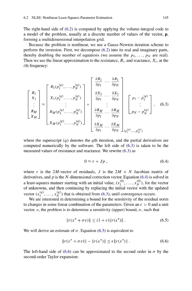
Because the problem is nonlinear, we use a Gauss-Newton iteration scheme to
perform the inversion. First, we decompose (6.2) into its real and imaginary parts,
thereby doubling the number of equations (we assume the p 1 , . . . , p N are real).
Then we use the linear approximation to the resistance, R i , and reactance, X i , at the
ith frequency:
⎡
⎢
⎢
⎢
⎢
⎢
⎢
⎣
R 1
X 1
. . .
R M
X M
⎤
⎥
⎥
⎥
⎥
⎥
⎥
⎦
≈
⎡
⎢
⎢
⎢
⎢
⎢
⎢
⎢
⎢
⎢
⎢
⎢
⎣
R 1 (p
(q)
1 , . . . , p
(q)
N )
X 1 (p
(q)
1 , . . . , p
(q)
N )
. . .
R M (p
(q)
1 , . . . , p
(q)
N )
X M (p
(q)
1 , . . . , p
(q)
N )
⎤
⎥
⎥
⎥
⎥
⎥
⎥
⎥
⎥
⎥
⎥
⎥
⎦
+
⎡
⎢
⎢
⎢
⎢
⎢
⎢
⎢
⎢
⎢
⎢
⎢
⎢
⎢
⎢
⎢
⎢
⎢
⎣
∂R 1
∂p 1
· · ·
∂R 1
∂p N
∂X 1
∂p 1
· · ·
∂X 1
∂p N
. . .
∂R M
∂p 1
· · ·
∂R M
∂p N
∂X M
∂p 1
· · ·
∂X M
∂p N
⎤
⎥
⎥
⎥
⎥
⎥
⎥
⎥
⎥
⎥
⎥
⎥
⎥
⎥
⎥
⎥
⎥
⎥
⎦
(p
(q)
1 ,...,p
(q)
N )
⎡
⎢
⎢
⎣
p 1 − p
(q)
1
. . .
p N − p
(q)
N
⎤
⎥
⎥
⎦ , (6.3)
where the superscript (q) denotes the qth iteration, and the partial derivatives are
computed numerically by the software. The left side of (6.3) is taken to be the
measured values of resistance and reactance. We rewrite (6.3) as
0 ≈ r + Jp ,
(6.4)
where r is the 2M-vector of residuals, J is the 2M × N Jacobian matrix of
derivatives, and p is the N-dimensional correction vector. Equation (6.4) is solved in
a least-squares manner starting with an initial value, (x
(0)
1 , . . . , x
(0)
N ), for the vector
of unknowns, and then continuing by replacing the initial vector with the updated
vector (x
(q)
1 , . . . , x
(q)
N ) that is obtained from (6.3), until convergence occurs.
We are interested in determining a bound for the sensitivity of the residual norm
to changes in some linear combination of the parameters. Given an > 0 and a unit
vector, v, the problem is to determine a sensitivity (upper) bound, σ , such that
r(x
∗
+ σ v) ≤ (1 + )r(x
∗ ) .
(6.5)
We will derive an estimate of σ . Equation (6.5) is equivalent to
r(x
∗
+ σ v) − −r(x
∗ ) ≤ r(x
∗ ) .
(6.6)
The left-hand side of (6.6) can be approximated to the second order in σ by the
second-order Taylor expansion:
145
The right-hand side of (6.2) is computed by applying the volume-integral code to
a model of the problem, usually at a discrete number of values of the vector, p,
forming a multidimensional interpolation grid.
Because the problem is nonlinear, we use a Gauss-Newton iteration scheme to
perform the inversion. First, we decompose (6.2) into its real and imaginary parts,
thereby doubling the number of equations (we assume the p 1 , . . . , p N are real).
Then we use the linear approximation to the resistance, R i , and reactance, X i , at the
ith frequency:
⎡
⎢
⎢
⎢
⎢
⎢
⎢
⎣
R 1
X 1
. . .
R M
X M
⎤
⎥
⎥
⎥
⎥
⎥
⎥
⎦
≈
⎡
⎢
⎢
⎢
⎢
⎢
⎢
⎢
⎢
⎢
⎢
⎢
⎣
R 1 (p
(q)
1 , . . . , p
(q)
N )
X 1 (p
(q)
1 , . . . , p
(q)
N )
. . .
R M (p
(q)
1 , . . . , p
(q)
N )
X M (p
(q)
1 , . . . , p
(q)
N )
⎤
⎥
⎥
⎥
⎥
⎥
⎥
⎥
⎥
⎥
⎥
⎥
⎦
+
⎡
⎢
⎢
⎢
⎢
⎢
⎢
⎢
⎢
⎢
⎢
⎢
⎢
⎢
⎢
⎢
⎢
⎢
⎣
∂R 1
∂p 1
· · ·
∂R 1
∂p N
∂X 1
∂p 1
· · ·
∂X 1
∂p N
. . .
∂R M
∂p 1
· · ·
∂R M
∂p N
∂X M
∂p 1
· · ·
∂X M
∂p N
⎤
⎥
⎥
⎥
⎥
⎥
⎥
⎥
⎥
⎥
⎥
⎥
⎥
⎥
⎥
⎥
⎥
⎥
⎦
(p
(q)
1 ,...,p
(q)
N )
⎡
⎢
⎢
⎣
p 1 − p
(q)
1
. . .
p N − p
(q)
N
⎤
⎥
⎥
⎦ , (6.3)
where the superscript (q) denotes the qth iteration, and the partial derivatives are
computed numerically by the software. The left side of (6.3) is taken to be the
measured values of resistance and reactance. We rewrite (6.3) as
0 ≈ r + Jp ,
(6.4)
where r is the 2M-vector of residuals, J is the 2M × N Jacobian matrix of
derivatives, and p is the N-dimensional correction vector. Equation (6.4) is solved in
a least-squares manner starting with an initial value, (x
(0)
1 , . . . , x
(0)
N ), for the vector
of unknowns, and then continuing by replacing the initial vector with the updated
vector (x
(q)
1 , . . . , x
(q)
N ) that is obtained from (6.3), until convergence occurs.
We are interested in determining a bound for the sensitivity of the residual norm
to changes in some linear combination of the parameters. Given an > 0 and a unit
vector, v, the problem is to determine a sensitivity (upper) bound, σ , such that
r(x
∗
+ σ v) ≤ (1 + )r(x
∗ ) .
(6.5)
We will derive an estimate of σ . Equation (6.5) is equivalent to
r(x
∗
+ σ v) − −r(x
∗ ) ≤ r(x
∗ ) .
(6.6)
The left-hand side of (6.6) can be approximated to the second order in σ by the
second-order Taylor expansion: