

144
6 Stochastic Inverse Problems: Models and Metrics
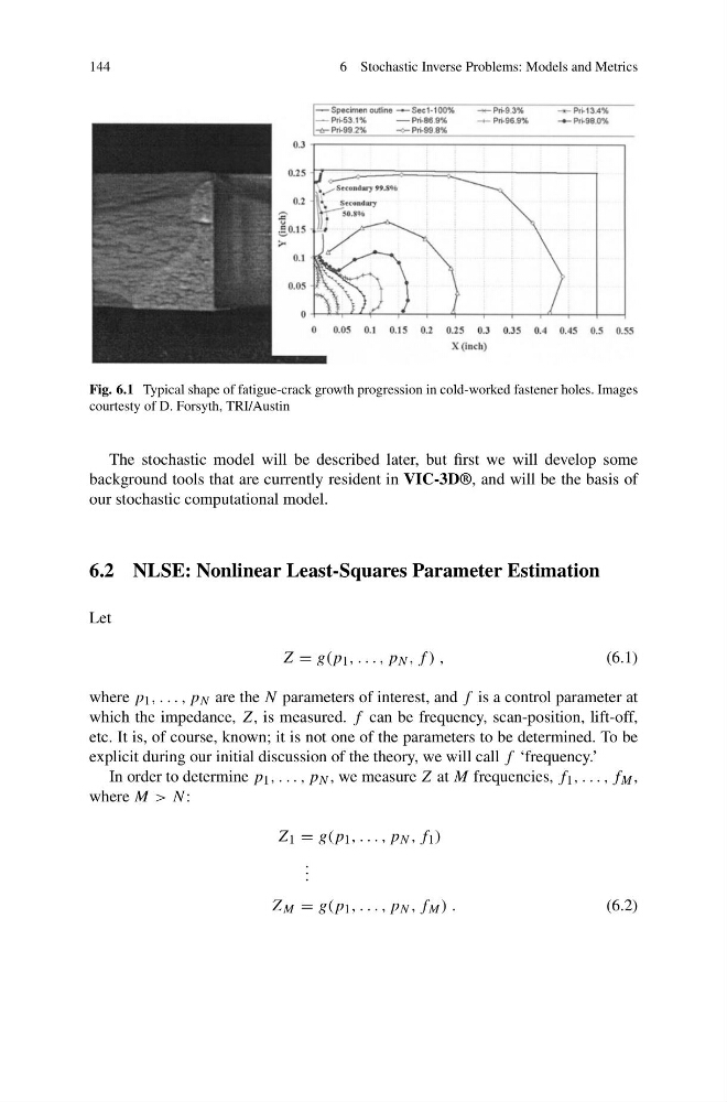
Fig. 6.1 Typical shape of fatigue-crack growth progression in cold-worked fastener holes. Images
courtesty of D. Forsyth, TRI/Austin
The stochastic model will be described later, but first we will develop some
background tools that are currently resident in VIC-3D®, and will be the basis of
our stochastic computational model.
6.2 NLSE: Nonlinear Least-Squares Parameter Estimation
Let
Z = g(p 1 , . . . , p N , f ) ,
(6.1)
where p 1 , . . . , p N are the N parameters of interest, and f is a control parameter at
which the impedance, Z, is measured. f can be frequency, scan-position, lift-off,
etc. It is, of course, known; it is not one of the parameters to be determined. To be
explicit during our initial discussion of the theory, we will call f ‘frequency.’
In order to determine p 1 , . . . , p N , we measure Z at M frequencies, f 1 , . . . , f M ,
where M > N:
Z 1 = g(p 1 , . . . , p N , f 1 )
. . .
Z M = g(p 1 , . . . , p N , f M ) .
(6.2)
6 Stochastic Inverse Problems: Models and Metrics
Fig. 6.1 Typical shape of fatigue-crack growth progression in cold-worked fastener holes. Images
courtesty of D. Forsyth, TRI/Austin
The stochastic model will be described later, but first we will develop some
background tools that are currently resident in VIC-3D®, and will be the basis of
our stochastic computational model.
6.2 NLSE: Nonlinear Least-Squares Parameter Estimation
Let
Z = g(p 1 , . . . , p N , f ) ,
(6.1)
where p 1 , . . . , p N are the N parameters of interest, and f is a control parameter at
which the impedance, Z, is measured. f can be frequency, scan-position, lift-off,
etc. It is, of course, known; it is not one of the parameters to be determined. To be
explicit during our initial discussion of the theory, we will call f ‘frequency.’
In order to determine p 1 , . . . , p N , we measure Z at M frequencies, f 1 , . . . , f M ,
where M > N:
Z 1 = g(p 1 , . . . , p N , f 1 )
. . .
Z M = g(p 1 , . . . , p N , f M ) .
(6.2)