

5.3 Some Inverse Problems with Random Anisotropies
135
-1
-0.5
0
0.5
1
1.5
2
2.5
3
0
0.5
1
1.5
2
2.5
3
R
Frequency (MHz)
Frequency Response of Racetrack Coil With a Ferrite Core
0 degrees
90 degrees
0
2
4
6
8
10
12
0
0.5
1
1.5
2
2.5
3
X
Frequency (MHz)
Frequency Response of Racetrack Coil With a Ferrite Core
0 degrees
90 degrees
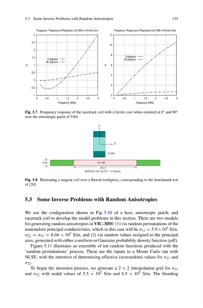
Fig. 5.7 Frequency response of the racetrack coil with a ferrite core when oriented at 0 ◦ and 90 ◦
over the anisotropic patch of Ti64
FLAW
101.0
WIDTH OF SLOT = 0.30mm
0.90
X
Y
COIL
Fig. 5.8 Illustrating a tangent coil over a flawed workpiece, corresponding to the benchmark test
of [20]
5.3 Some Inverse Problems with Random Anisotropies
We use the configuration shown in Fig. 5.10 of a host, anisotropic patch, and
racetrack coil to develop the model problems in this section. There are two models
for generating random anisotropies in VIC-3D®: (1) via random permutations of the
nonrandom principal conductivities, which in this case will be σ 11 = 5.9 × 10 5 S/m,
σ 22 = σ 33 = 6.04 × 10 5 S/m, and (2) via random values assigned to the principal
axes, generated with either a uniform or Gaussian probability density function (pdf).
Figure 5.11 illustrates an ensemble of ten random functions produced with the
‘random permutations’ process. These are the inputs to a Monte Carlo run with
NLSE, with the intention of determining effective (nonrandom) values for σ 11 and
σ 22 .
To begin the inversion process, we generate a 2 × 2 interpolation grid for σ 11
and σ 22 with nodal values of 5.5 × 10 5 S/m and 6.5 × 10 5 S/m. The blending
135
-1
-0.5
0
0.5
1
1.5
2
2.5
3
0
0.5
1
1.5
2
2.5
3
R
Frequency (MHz)
Frequency Response of Racetrack Coil With a Ferrite Core
0 degrees
90 degrees
0
2
4
6
8
10
12
0
0.5
1
1.5
2
2.5
3
X
Frequency (MHz)
Frequency Response of Racetrack Coil With a Ferrite Core
0 degrees
90 degrees
Fig. 5.7 Frequency response of the racetrack coil with a ferrite core when oriented at 0 ◦ and 90 ◦
over the anisotropic patch of Ti64
FLAW
101.0
WIDTH OF SLOT = 0.30mm
0.90
X
Y
COIL
Fig. 5.8 Illustrating a tangent coil over a flawed workpiece, corresponding to the benchmark test
of [20]
5.3 Some Inverse Problems with Random Anisotropies
We use the configuration shown in Fig. 5.10 of a host, anisotropic patch, and
racetrack coil to develop the model problems in this section. There are two models
for generating random anisotropies in VIC-3D®: (1) via random permutations of the
nonrandom principal conductivities, which in this case will be σ 11 = 5.9 × 10 5 S/m,
σ 22 = σ 33 = 6.04 × 10 5 S/m, and (2) via random values assigned to the principal
axes, generated with either a uniform or Gaussian probability density function (pdf).
Figure 5.11 illustrates an ensemble of ten random functions produced with the
‘random permutations’ process. These are the inputs to a Monte Carlo run with
NLSE, with the intention of determining effective (nonrandom) values for σ 11 and
σ 22 .
To begin the inversion process, we generate a 2 × 2 interpolation grid for σ 11
and σ 22 with nodal values of 5.5 × 10 5 S/m and 6.5 × 10 5 S/m. The blending