

134
5 An Electromagnetic Model for Anisotropic Media: Green’s Dyad for Plane-. . .
-25
-20
-15
-10
-5
0
5
10
15
0.5
1
1.5
2
2.5
3
Ohms
Frequency (MHz)
DeltaZ of Racetrack Coil Over Ti64: Parallel/Perpendicular Alignment
R(par)
R(perp)
X(par)
X(perp)
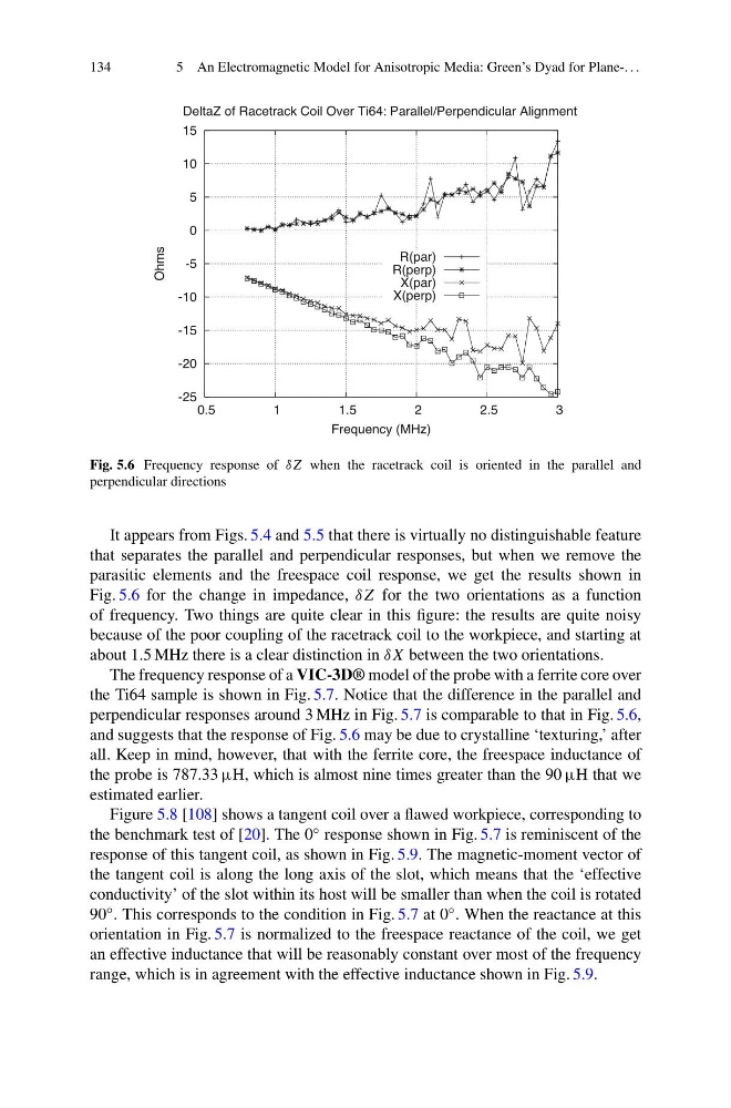
Fig. 5.6 Frequency response of δZ when the racetrack coil is oriented in the parallel and
perpendicular directions
It appears from Figs. 5.4 and 5.5 that there is virtually no distinguishable feature
that separates the parallel and perpendicular responses, but when we remove the
parasitic elements and the freespace coil response, we get the results shown in
Fig. 5.6 for the change in impedance, δZ for the two orientations as a function
of frequency. Two things are quite clear in this figure: the results are quite noisy
because of the poor coupling of the racetrack coil to the workpiece, and starting at
about 1.5 MHz there is a clear distinction in δX between the two orientations.
The frequency response of a VIC-3D® model of the probe with a ferrite core over
the Ti64 sample is shown in Fig. 5.7. Notice that the difference in the parallel and
perpendicular responses around 3 MHz in Fig. 5.7 is comparable to that in Fig. 5.6,
and suggests that the response of Fig. 5.6 may be due to crystalline ‘texturing,’ after
all. Keep in mind, however, that with the ferrite core, the freespace inductance of
the probe is 787.33 µH, which is almost nine times greater than the 90 µH that we
estimated earlier.
Figure 5.8 [108] shows a tangent coil over a flawed workpiece, corresponding to
the benchmark test of [20]. The 0 ◦ response shown in Fig. 5.7 is reminiscent of the
response of this tangent coil, as shown in Fig. 5.9. The magnetic-moment vector of
the tangent coil is along the long axis of the slot, which means that the ‘effective
conductivity’ of the slot within its host will be smaller than when the coil is rotated
90 ◦ . This corresponds to the condition in Fig. 5.7 at 0 ◦ . When the reactance at this
orientation in Fig. 5.7 is normalized to the freespace reactance of the coil, we get
an effective inductance that will be reasonably constant over most of the frequency
range, which is in agreement with the effective inductance shown in Fig. 5.9.
5 An Electromagnetic Model for Anisotropic Media: Green’s Dyad for Plane-. . .
-25
-20
-15
-10
-5
0
5
10
15
0.5
1
1.5
2
2.5
3
Ohms
Frequency (MHz)
DeltaZ of Racetrack Coil Over Ti64: Parallel/Perpendicular Alignment
R(par)
R(perp)
X(par)
X(perp)
Fig. 5.6 Frequency response of δZ when the racetrack coil is oriented in the parallel and
perpendicular directions
It appears from Figs. 5.4 and 5.5 that there is virtually no distinguishable feature
that separates the parallel and perpendicular responses, but when we remove the
parasitic elements and the freespace coil response, we get the results shown in
Fig. 5.6 for the change in impedance, δZ for the two orientations as a function
of frequency. Two things are quite clear in this figure: the results are quite noisy
because of the poor coupling of the racetrack coil to the workpiece, and starting at
about 1.5 MHz there is a clear distinction in δX between the two orientations.
The frequency response of a VIC-3D® model of the probe with a ferrite core over
the Ti64 sample is shown in Fig. 5.7. Notice that the difference in the parallel and
perpendicular responses around 3 MHz in Fig. 5.7 is comparable to that in Fig. 5.6,
and suggests that the response of Fig. 5.6 may be due to crystalline ‘texturing,’ after
all. Keep in mind, however, that with the ferrite core, the freespace inductance of
the probe is 787.33 µH, which is almost nine times greater than the 90 µH that we
estimated earlier.
Figure 5.8 [108] shows a tangent coil over a flawed workpiece, corresponding to
the benchmark test of [20]. The 0 ◦ response shown in Fig. 5.7 is reminiscent of the
response of this tangent coil, as shown in Fig. 5.9. The magnetic-moment vector of
the tangent coil is along the long axis of the slot, which means that the ‘effective
conductivity’ of the slot within its host will be smaller than when the coil is rotated
90 ◦ . This corresponds to the condition in Fig. 5.7 at 0 ◦ . When the reactance at this
orientation in Fig. 5.7 is normalized to the freespace reactance of the coil, we get
an effective inductance that will be reasonably constant over most of the frequency
range, which is in agreement with the effective inductance shown in Fig. 5.9.