

136
5 An Electromagnetic Model for Anisotropic Media: Green’s Dyad for Plane-. . .
-6
-4
-2
0
2
4
6
8
10
12
0
1000
2000
3000
4000
5000
6000
7000
8000
9000 10000
Inductance (mH) or Resistance (Ohms)
f(Hz)
RESULTS FOR TANGENT COIL OVER SLOT
L(data)
L(Vic3D)
R(data)
R(Vic3D)
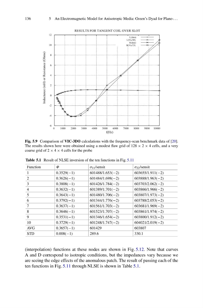
Fig. 5.9 Comparison of VIC-3D® calculations with the frequency-scan benchmark data of [20].
The results shown here were obtained using a modest flaw grid of 128 × 2 × 4 cells, and a very
coarse grid of 2 × 4 × 4 cells for the probe
Table 5.1 Result of NLSE inversion of the ten functions in Fig. 5.11
Function
Φ
σ 11 /sensit
σ 22 /sensit
1
0.3529(−1)
601488/1.653(−2)
603655/1.911(−2)
2
0.3626(−1)
601484/1.698(−2)
603888/1.963(−2)
3
0.3808(−1)
601426/1.784(−2)
603703/2.062(−2)
4
0.3632(−1)
601389/1.701(−2)
603866/1.966(−2)
5
0.3643(−1)
601480/1.706(−2)
603807/1.973(−2)
6
0.3792(−1)
601344/1.776(−2)
603788/2.053(−2)
7
0.3637(−1)
601561/1.703(−2)
603681/1.969(−2)
8
0.3646(−1)
601523/1.707(−2)
603861/1.974(−2)
9
0.3531(−1)
601346/1.654(−2)
603800/1.912(−2)
10
0.3729(−1)
601248/1.747(−2)
604021/2.019(−2)
AVG
0.3657(−1)
601429
603807
STD
0.008(−1)
289.6
330.1
(interpolation) functions at these nodes are shown in Fig. 5.12. Note that curves
A and D correspond to isotropic conditions, but the impedances vary because we
are seeing the edge effects of the anomalous patch. The result of passing each of the
ten functions in Fig. 5.11 through NLSE is shown in Table 5.1.
5 An Electromagnetic Model for Anisotropic Media: Green’s Dyad for Plane-. . .
-6
-4
-2
0
2
4
6
8
10
12
0
1000
2000
3000
4000
5000
6000
7000
8000
9000 10000
Inductance (mH) or Resistance (Ohms)
f(Hz)
RESULTS FOR TANGENT COIL OVER SLOT
L(data)
L(Vic3D)
R(data)
R(Vic3D)
Fig. 5.9 Comparison of VIC-3D® calculations with the frequency-scan benchmark data of [20].
The results shown here were obtained using a modest flaw grid of 128 × 2 × 4 cells, and a very
coarse grid of 2 × 4 × 4 cells for the probe
Table 5.1 Result of NLSE inversion of the ten functions in Fig. 5.11
Function
Φ
σ 11 /sensit
σ 22 /sensit
1
0.3529(−1)
601488/1.653(−2)
603655/1.911(−2)
2
0.3626(−1)
601484/1.698(−2)
603888/1.963(−2)
3
0.3808(−1)
601426/1.784(−2)
603703/2.062(−2)
4
0.3632(−1)
601389/1.701(−2)
603866/1.966(−2)
5
0.3643(−1)
601480/1.706(−2)
603807/1.973(−2)
6
0.3792(−1)
601344/1.776(−2)
603788/2.053(−2)
7
0.3637(−1)
601561/1.703(−2)
603681/1.969(−2)
8
0.3646(−1)
601523/1.707(−2)
603861/1.974(−2)
9
0.3531(−1)
601346/1.654(−2)
603800/1.912(−2)
10
0.3729(−1)
601248/1.747(−2)
604021/2.019(−2)
AVG
0.3657(−1)
601429
603807
STD
0.008(−1)
289.6
330.1
(interpolation) functions at these nodes are shown in Fig. 5.12. Note that curves
A and D correspond to isotropic conditions, but the impedances vary because we
are seeing the edge effects of the anomalous patch. The result of passing each of the
ten functions in Fig. 5.11 through NLSE is shown in Table 5.1.