

120
4 Application of the Set-Theoretic Algorithm to CFRP’s
-150000
-100000
-50000
0
50000
100000
150000
200000
250000
300000
-3000 -2500 -2000 -1500 -1000 -500
0
500 1000 1500
Jy
Ey
Anomalous Conductivity for (k,l,m) = (3,3,2)
Real
Imag
Jy = -100.0*Ey
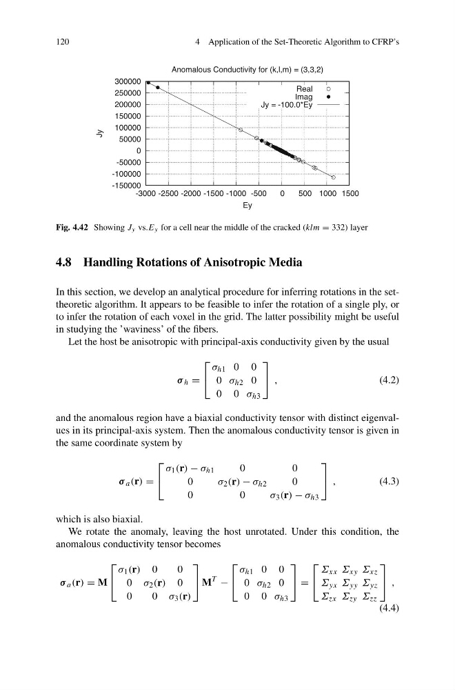
Fig. 4.42 Showing J y vs.E y for a cell near the middle of the cracked (klm = 332) layer
4.8 Handling Rotations of Anisotropic Media
In this section, we develop an analytical procedure for inferring rotations in the settheoretic algorithm. It appears to be feasible to infer the rotation of a single ply, or
to infer the rotation of each voxel in the grid. The latter possibility might be useful
in studying the ’waviness’ of the fibers.
Let the host be anisotropic with principal-axis conductivity given by the usual
σ h =
⎡
⎣
σ h1 0 0
0 σ h2 0
0 0 σ h3
⎤
⎦ ,
(4.2)
and the anomalous region have a biaxial conductivity tensor with distinct eigenvalues in its principal-axis system. Then the anomalous conductivity tensor is given in
the same coordinate system by
σ a (r) =
⎡
⎣
σ 1 (r) − σ h1
0
0
0
σ 2 (r) − σ h2
0
0
0
σ 3 (r) − σ h3
⎤
⎦ ,
(4.3)
which is also biaxial.
We rotate the anomaly, leaving the host unrotated. Under this condition, the
anomalous conductivity tensor becomes
σ a (r) = M
⎡
⎣
σ 1 (r) 0
0
0 σ 2 (r) 0
0
0 σ 3 (r)
⎤
⎦ M
T
−
⎡
⎣
σ h1 0 0
0 σ h2 0
0 0 σ h3
⎤
⎦ =
⎡
⎣
Σ xx Σ xy Σ xz
Σ yx Σ yy Σ yz
Σ zx Σ zy Σ zz
⎤
⎦ ,
(4.4)
4 Application of the Set-Theoretic Algorithm to CFRP’s
-150000
-100000
-50000
0
50000
100000
150000
200000
250000
300000
-3000 -2500 -2000 -1500 -1000 -500
0
500 1000 1500
Jy
Ey
Anomalous Conductivity for (k,l,m) = (3,3,2)
Real
Imag
Jy = -100.0*Ey
Fig. 4.42 Showing J y vs.E y for a cell near the middle of the cracked (klm = 332) layer
4.8 Handling Rotations of Anisotropic Media
In this section, we develop an analytical procedure for inferring rotations in the settheoretic algorithm. It appears to be feasible to infer the rotation of a single ply, or
to infer the rotation of each voxel in the grid. The latter possibility might be useful
in studying the ’waviness’ of the fibers.
Let the host be anisotropic with principal-axis conductivity given by the usual
σ h =
⎡
⎣
σ h1 0 0
0 σ h2 0
0 0 σ h3
⎤
⎦ ,
(4.2)
and the anomalous region have a biaxial conductivity tensor with distinct eigenvalues in its principal-axis system. Then the anomalous conductivity tensor is given in
the same coordinate system by
σ a (r) =
⎡
⎣
σ 1 (r) − σ h1
0
0
0
σ 2 (r) − σ h2
0
0
0
σ 3 (r) − σ h3
⎤
⎦ ,
(4.3)
which is also biaxial.
We rotate the anomaly, leaving the host unrotated. Under this condition, the
anomalous conductivity tensor becomes
σ a (r) = M
⎡
⎣
σ 1 (r) 0
0
0 σ 2 (r) 0
0
0 σ 3 (r)
⎤
⎦ M
T
−
⎡
⎣
σ h1 0 0
0 σ h2 0
0 0 σ h3
⎤
⎦ =
⎡
⎣
Σ xx Σ xy Σ xz
Σ yx Σ yy Σ yz
Σ zx Σ zy Σ zz
⎤
⎦ ,
(4.4)