

100
4 Application of the Set-Theoretic Algorithm to CFRP’s
-1.5x10
6
-1x10
6
-500000
0
500000
1x10
6
1.5x10
6
-1000 -800
-600
-400
-200
0
200
400
Jx
Ex
Anomalous Conductivity for (k,l,m) = (3,3,3)
Real
Imag
Jx = 1262*Ex
-800000
-600000
-400000
-200000
0
200000
400000
600000
800000
1x10
6
-10000 -5000
0
5000
10000
15000
20000
Jy
Ey
Anomalous Conductivity for (k,l,m) = (3,3,3)
Real
Imag
Jy = -41*Ey
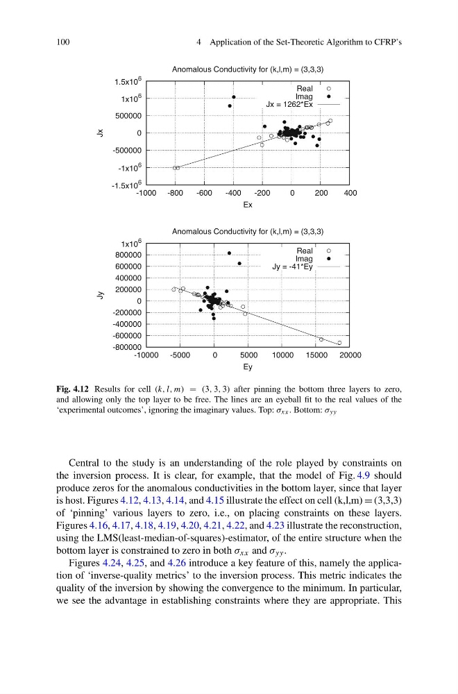
Fig. 4.12 Results for cell (k, l, m) = (3, 3, 3) after pinning the bottom three layers to zero,
and allowing only the top layer to be free. The lines are an eyeball fit to the real values of the
‘experimental outcomes’, ignoring the imaginary values. Top: σ xx . Bottom: σ yy
Central to the study is an understanding of the role played by constraints on
the inversion process. It is clear, for example, that the model of Fig. 4.9 should
produce zeros for the anomalous conductivities in the bottom layer, since that layer
is host. Figures 4.12, 4.13, 4.14, and 4.15 illustrate the effect on cell (k,l,m) = (3,3,3)
of ‘pinning’ various layers to zero, i.e., on placing constraints on these layers.
Figures 4.16, 4.17, 4.18, 4.19, 4.20, 4.21, 4.22, and 4.23 illustrate the reconstruction,
using the LMS(least-median-of-squares)-estimator, of the entire structure when the
bottom layer is constrained to zero in both σ xx and σ yy .
Figures 4.24, 4.25, and 4.26 introduce a key feature of this, namely the application of ‘inverse-quality metrics’ to the inversion process. This metric indicates the
quality of the inversion by showing the convergence to the minimum. In particular,
we see the advantage in establishing constraints where they are appropriate. This
4 Application of the Set-Theoretic Algorithm to CFRP’s
-1.5x10
6
-1x10
6
-500000
0
500000
1x10
6
1.5x10
6
-1000 -800
-600
-400
-200
0
200
400
Jx
Ex
Anomalous Conductivity for (k,l,m) = (3,3,3)
Real
Imag
Jx = 1262*Ex
-800000
-600000
-400000
-200000
0
200000
400000
600000
800000
1x10
6
-10000 -5000
0
5000
10000
15000
20000
Jy
Ey
Anomalous Conductivity for (k,l,m) = (3,3,3)
Real
Imag
Jy = -41*Ey
Fig. 4.12 Results for cell (k, l, m) = (3, 3, 3) after pinning the bottom three layers to zero,
and allowing only the top layer to be free. The lines are an eyeball fit to the real values of the
‘experimental outcomes’, ignoring the imaginary values. Top: σ xx . Bottom: σ yy
Central to the study is an understanding of the role played by constraints on
the inversion process. It is clear, for example, that the model of Fig. 4.9 should
produce zeros for the anomalous conductivities in the bottom layer, since that layer
is host. Figures 4.12, 4.13, 4.14, and 4.15 illustrate the effect on cell (k,l,m) = (3,3,3)
of ‘pinning’ various layers to zero, i.e., on placing constraints on these layers.
Figures 4.16, 4.17, 4.18, 4.19, 4.20, 4.21, 4.22, and 4.23 illustrate the reconstruction,
using the LMS(least-median-of-squares)-estimator, of the entire structure when the
bottom layer is constrained to zero in both σ xx and σ yy .
Figures 4.24, 4.25, and 4.26 introduce a key feature of this, namely the application of ‘inverse-quality metrics’ to the inversion process. This metric indicates the
quality of the inversion by showing the convergence to the minimum. In particular,
we see the advantage in establishing constraints where they are appropriate. This