

4.6 Advanced Features for Set-Theoretic Microstructure Quantification
101
-2x10
6
-1.5x10
6
-1x10
6
-500000
0
500000
1x10
6
-250
-200
-150
-100
-50
0
50
100
Jx
Ex
Anomalous Conductivity for (k,l,m) = (3,3,3)
Real
Imag
Jx = 6585*Ex
-800
-600
-400
-200
0
200
400
600
-10000 -5000
0
5000
10000
15000
20000
Jy
Ey
Anomalous Conductivity for (k,l,m) = (3,3,3)
Real
Imag
Jy = 0*Ey
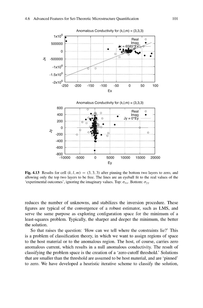
Fig. 4.13 Results for cell (k, l, m) = (3, 3, 3) after pinning the bottom two layers to zero, and
allowing only the top two layers to be free. The lines are an eyeball fit to the real values of the
‘experimental outcomes’, ignoring the imaginary values. Top: σ xx . Bottom: σ yy
reduces the number of unknowns, and stabilizes the inversion procedure. These
figures are typical of the convergence of a robust estimator, such as LMS, and
serve the same purpose as exploring configuration space for the minimum of a
least-squares problem. Typically, the sharper and deeper the minimum, the better
the solution.
So that raises the question: ‘How can we tell where the constraints lie?’ This
is a problem of classification theory, in which we want to assign regions of space
to the host material or to the anomalous region. The host, of course, carries zero
anomalous current, which results in a null anomalous conductivity. The result of
classifying the problem space is the creation of a ‘zero-cutoff threshold.’ Solutions
that are smaller than the threshold are assumed to be host material, and are ‘pinned’
to zero. We have developed a heuristic iterative scheme to classify the solution,
101
-2x10
6
-1.5x10
6
-1x10
6
-500000
0
500000
1x10
6
-250
-200
-150
-100
-50
0
50
100
Jx
Ex
Anomalous Conductivity for (k,l,m) = (3,3,3)
Real
Imag
Jx = 6585*Ex
-800
-600
-400
-200
0
200
400
600
-10000 -5000
0
5000
10000
15000
20000
Jy
Ey
Anomalous Conductivity for (k,l,m) = (3,3,3)
Real
Imag
Jy = 0*Ey
Fig. 4.13 Results for cell (k, l, m) = (3, 3, 3) after pinning the bottom two layers to zero, and
allowing only the top two layers to be free. The lines are an eyeball fit to the real values of the
‘experimental outcomes’, ignoring the imaginary values. Top: σ xx . Bottom: σ yy
reduces the number of unknowns, and stabilizes the inversion procedure. These
figures are typical of the convergence of a robust estimator, such as LMS, and
serve the same purpose as exploring configuration space for the minimum of a
least-squares problem. Typically, the sharper and deeper the minimum, the better
the solution.
So that raises the question: ‘How can we tell where the constraints lie?’ This
is a problem of classification theory, in which we want to assign regions of space
to the host material or to the anomalous region. The host, of course, carries zero
anomalous current, which results in a null anomalous conductivity. The result of
classifying the problem space is the creation of a ‘zero-cutoff threshold.’ Solutions
that are smaller than the threshold are assumed to be host material, and are ‘pinned’
to zero. We have developed a heuristic iterative scheme to classify the solution,