

4.6 Advanced Features for Set-Theoretic Microstructure Quantification
99
-0.04
-0.02
0
0.02
0.04
0.06
0.08
-2
-1.5
-1
-0.5
0
0.5
1
1.5
2
R
Scan Position (mm)
0.00
0.025
0.050
0
0.5
1
1.5
2
2.5
3
-2
-1.5
-1
-0.5
0
0.5
1
1.5
2
X
Scan Position (mm)
0.00
0.025
0.050
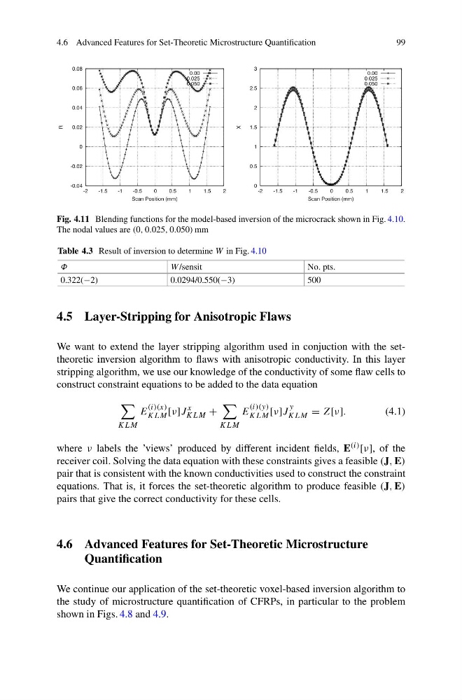
Fig. 4.11 Blending functions for the model-based inversion of the microcrack shown in Fig. 4.10.
The nodal values are (0, 0.025, 0.050) mm
Table 4.3 Result of inversion to determine W in Fig. 4.10
Φ
W /sensit
No. pts.
0.322(−2)
0.0294/0.550(−3)
500
4.5 Layer-Stripping for Anisotropic Flaws
We want to extend the layer stripping algorithm used in conjuction with the settheoretic inversion algorithm to flaws with anisotropic conductivity. In this layer
stripping algorithm, we use our knowledge of the conductivity of some flaw cells to
construct constraint equations to be added to the data equation
KLM
E
(i)(x)
KLM [ν]J
x
KLM +
KLM
E
(i)(y)
KLM [ν]J
y
KLM = Z[ν].
(4.1)
where ν labels the ’views’ produced by different incident fields, E (i) [ν], of the
receiver coil. Solving the data equation with these constraints gives a feasible (J, E)
pair that is consistent with the known conductivities used to construct the constraint
equations. That is, it forces the set-theoretic algorithm to produce feasible (J, E)
pairs that give the correct conductivity for these cells.
4.6 Advanced Features for Set-Theoretic Microstructure
Quantification
We continue our application of the set-theoretic voxel-based inversion algorithm to
the study of microstructure quantification of CFRPs, in particular to the problem
shown in Figs. 4.8 and 4.9.
99
-0.04
-0.02
0
0.02
0.04
0.06
0.08
-2
-1.5
-1
-0.5
0
0.5
1
1.5
2
R
Scan Position (mm)
0.00
0.025
0.050
0
0.5
1
1.5
2
2.5
3
-2
-1.5
-1
-0.5
0
0.5
1
1.5
2
X
Scan Position (mm)
0.00
0.025
0.050
Fig. 4.11 Blending functions for the model-based inversion of the microcrack shown in Fig. 4.10.
The nodal values are (0, 0.025, 0.050) mm
Table 4.3 Result of inversion to determine W in Fig. 4.10
Φ
W /sensit
No. pts.
0.322(−2)
0.0294/0.550(−3)
500
4.5 Layer-Stripping for Anisotropic Flaws
We want to extend the layer stripping algorithm used in conjuction with the settheoretic inversion algorithm to flaws with anisotropic conductivity. In this layer
stripping algorithm, we use our knowledge of the conductivity of some flaw cells to
construct constraint equations to be added to the data equation
KLM
E
(i)(x)
KLM [ν]J
x
KLM +
KLM
E
(i)(y)
KLM [ν]J
y
KLM = Z[ν].
(4.1)
where ν labels the ’views’ produced by different incident fields, E (i) [ν], of the
receiver coil. Solving the data equation with these constraints gives a feasible (J, E)
pair that is consistent with the known conductivities used to construct the constraint
equations. That is, it forces the set-theoretic algorithm to produce feasible (J, E)
pairs that give the correct conductivity for these cells.
4.6 Advanced Features for Set-Theoretic Microstructure
Quantification
We continue our application of the set-theoretic voxel-based inversion algorithm to
the study of microstructure quantification of CFRPs, in particular to the problem
shown in Figs. 4.8 and 4.9.