

3.4 Experimental Implementation of RP-THz-TDS
61
3.4.3.1 Rotating the Frame of Reference
As Figs. 3.8 and 3.9 have shown, the polarisation state of the THz pulses experiences
no change when the electric field is parallel to a polarisation eigenvector in the
sample. The transmitted THz pulse therefore has the same orientation angle as the
incident pulse; if the frame of reference of the sample and reference pulses can be
rotated to match that of the polarisation eigenvector, then the usual one-dimensional
data analysis to extract n(ω) and α(ω) as described in Sect. 2.4.1 can be applied.
The rotation matrix R representing points in the cartesian x-y plane being rotated
anticlockwise about the orgin of the coordinate system by an angle θ R is
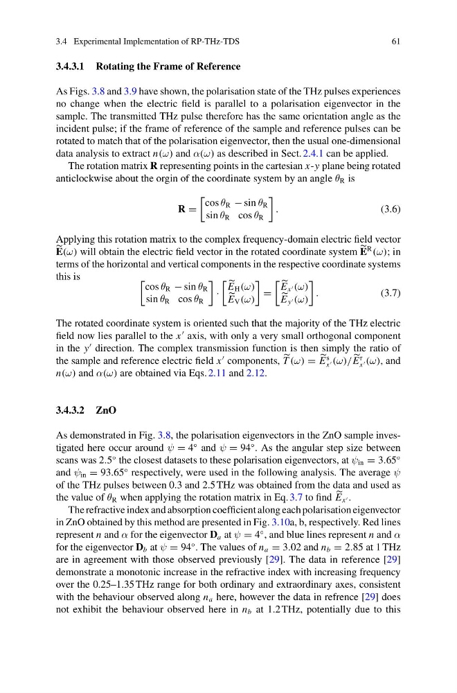
R =
cos θ R − sin θ R
sin θ R cos θ R
.
(3.6)
Applying this rotation matrix to the complex frequency-domain electric field vector
E(ω) will obtain the electric field vector in the rotated coordinate system E
R
(ω); in
terms of the horizontal and vertical components in the respective coordinate systems
this is
cos θ R − sin θ R
sin θ R cos θ R
·
E H (ω)
E V (ω)
=
E x (ω)
E y (ω)
.
(3.7)
The rotated coordinate system is oriented such that the majority of the THz electric
field now lies parallel to the x
axis, with only a very small orthogonal component
in the y
direction. The complex transmission function is then simply the ratio of
the sample and reference electric field x
components,
T (ω) =
E
s
x (ω)/
E
r
x (ω), and
n(ω) and α(ω) are obtained via Eqs. 2.11 and 2.12.
3.4.3.2 ZnO
As demonstrated in Fig. 3.8, the polarisation eigenvectors in the ZnO sample investigated here occur around ψ = 4
◦ and ψ = 94
◦ . As the angular step size between
scans was 2.5
◦ the closest datasets to these polarisation eigenvectors, at ψ in = 3.65
◦
and ψ in = 93.65
◦ respectively, were used in the following analysis. The average ψ
of the THz pulses between 0.3 and 2.5 THz was obtained from the data and used as
the value of θ R when applying the rotation matrix in Eq. 3.7 to find
E x .
The refractive index and absorption coefficient along each polarisation eigenvector
in ZnO obtained by this method are presented in Fig. 3.10a, b, respectively. Red lines
represent n and α for the eigenvector D a at ψ = 4
◦ , and blue lines represent n and α
for the eigenvector D b at ψ = 94
◦ . The values of n a = 3.02 and n b = 2.85 at 1 THz
are in agreement with those observed previously [29]. The data in reference [29]
demonstrate a monotonic increase in the refractive index with increasing frequency
over the 0.25–1.35 THz range for both ordinary and extraordinary axes, consistent
with the behaviour observed along n a here, however the data in refrence [29] does
not exhibit the behaviour observed here in n b at 1.2 THz, potentially due to this
61
3.4.3.1 Rotating the Frame of Reference
As Figs. 3.8 and 3.9 have shown, the polarisation state of the THz pulses experiences
no change when the electric field is parallel to a polarisation eigenvector in the
sample. The transmitted THz pulse therefore has the same orientation angle as the
incident pulse; if the frame of reference of the sample and reference pulses can be
rotated to match that of the polarisation eigenvector, then the usual one-dimensional
data analysis to extract n(ω) and α(ω) as described in Sect. 2.4.1 can be applied.
The rotation matrix R representing points in the cartesian x-y plane being rotated
anticlockwise about the orgin of the coordinate system by an angle θ R is
R =
cos θ R − sin θ R
sin θ R cos θ R
.
(3.6)
Applying this rotation matrix to the complex frequency-domain electric field vector
E(ω) will obtain the electric field vector in the rotated coordinate system E
R
(ω); in
terms of the horizontal and vertical components in the respective coordinate systems
this is
cos θ R − sin θ R
sin θ R cos θ R
·
E H (ω)
E V (ω)
=
E x (ω)
E y (ω)
.
(3.7)
The rotated coordinate system is oriented such that the majority of the THz electric
field now lies parallel to the x
axis, with only a very small orthogonal component
in the y
direction. The complex transmission function is then simply the ratio of
the sample and reference electric field x
components,
T (ω) =
E
s
x (ω)/
E
r
x (ω), and
n(ω) and α(ω) are obtained via Eqs. 2.11 and 2.12.
3.4.3.2 ZnO
As demonstrated in Fig. 3.8, the polarisation eigenvectors in the ZnO sample investigated here occur around ψ = 4
◦ and ψ = 94
◦ . As the angular step size between
scans was 2.5
◦ the closest datasets to these polarisation eigenvectors, at ψ in = 3.65
◦
and ψ in = 93.65
◦ respectively, were used in the following analysis. The average ψ
of the THz pulses between 0.3 and 2.5 THz was obtained from the data and used as
the value of θ R when applying the rotation matrix in Eq. 3.7 to find
E x .
The refractive index and absorption coefficient along each polarisation eigenvector
in ZnO obtained by this method are presented in Fig. 3.10a, b, respectively. Red lines
represent n and α for the eigenvector D a at ψ = 4
◦ , and blue lines represent n and α
for the eigenvector D b at ψ = 94
◦ . The values of n a = 3.02 and n b = 2.85 at 1 THz
are in agreement with those observed previously [29]. The data in reference [29]
demonstrate a monotonic increase in the refractive index with increasing frequency
over the 0.25–1.35 THz range for both ordinary and extraordinary axes, consistent
with the behaviour observed along n a here, however the data in refrence [29] does
not exhibit the behaviour observed here in n b at 1.2 THz, potentially due to this