

88
7 Regression Models and Hypothesis Testing
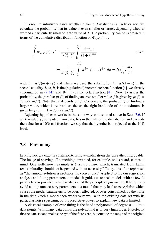
In order to intuitively asses whether a found f -statistics is likely or not, we
calculate the probability that its value is even smaller or larger, depending whether
we find a particularly small or large value of f . The probability can be expressed in
terms of the cumulative distribution function of n,m ( f ) by
f
0
n,m ( f
)d f
=
1
B
n
2
,
m
2
n
m f
0
t
n
2 −1 dt
(1 + t)
n+m
2
(7.43)
=
1
B
n
2
,
m
2
n f
m+n f
0
u
n
2 −1
(1 − u)
m
2 −1 du = I ˆ
x
n
2
,
m
2
with ˆ
x = n f/(m + n f ) and where we used the substitution t = u/(1 − u) in the
second equality. I ˆ
x (a, b) is the (regularized) incomplete beta function [4], we already
encountered in (7.34), and B(a, b) is the beta function [4]. Now, to assess the
probability, the p-value p( f ), of finding an even smaller value f is given by p( f ) =
I ˆ
x (n/2, m/2). Note that ˆ
x depends on f . Conversely, the probability of finding a
larger value, which is relevant on the on the right-hand side of the maximum, is
given by p( f ) = 1 − I ˆ
x (n/2, m/2).
Rejecting hypotheses works in the same way as discussed above in Sect. 7.6. If
an F−value f , computed from data, lies in the tails of the distribution and exceeds
the value for a 10% tail-fraction, we say that the hypothesis is rejected at the 10%
level.
7.8 Parsimony
In philosophy, a razor is a criterion to remove explanations that are rather improbable.
The image of shaving off something unwanted, for example, one’s beard, comes to
mind. One well-known example is Occam’s razor, which, translated from Latin,
reads “plurality should not be posited without necessity.” Today, it is often rephrased
as “the simpler solution is probably the correct one.” Applied to the our regression
analysis and fitting parameters to models it guides us to seek models with as few fit
parameters as possible, which is also called the principle of parsimony. It helps us to
avoid adding unnecessary parameters to a model that may lead to over-fitting which
causes the model parameters to be overly affected, or over-constrained, by the noise
in the data. Such a model then works very well with the existing data set with its
particular noise spectrum, but its predictive power to explain new data is limited.
A classical example of over-fitting is the fit of a polynomial of degree n − 1 to n
data points. With many data points the polynomial is of very high order. It perfectly
fits the data set and makes the χ
2 of the fit to zero, but outside the range of the original
7 Regression Models and Hypothesis Testing
In order to intuitively asses whether a found f -statistics is likely or not, we
calculate the probability that its value is even smaller or larger, depending whether
we find a particularly small or large value of f . The probability can be expressed in
terms of the cumulative distribution function of n,m ( f ) by
f
0
n,m ( f
)d f
=
1
B
n
2
,
m
2
n
m f
0
t
n
2 −1 dt
(1 + t)
n+m
2
(7.43)
=
1
B
n
2
,
m
2
n f
m+n f
0
u
n
2 −1
(1 − u)
m
2 −1 du = I ˆ
x
n
2
,
m
2
with ˆ
x = n f/(m + n f ) and where we used the substitution t = u/(1 − u) in the
second equality. I ˆ
x (a, b) is the (regularized) incomplete beta function [4], we already
encountered in (7.34), and B(a, b) is the beta function [4]. Now, to assess the
probability, the p-value p( f ), of finding an even smaller value f is given by p( f ) =
I ˆ
x (n/2, m/2). Note that ˆ
x depends on f . Conversely, the probability of finding a
larger value, which is relevant on the on the right-hand side of the maximum, is
given by p( f ) = 1 − I ˆ
x (n/2, m/2).
Rejecting hypotheses works in the same way as discussed above in Sect. 7.6. If
an F−value f , computed from data, lies in the tails of the distribution and exceeds
the value for a 10% tail-fraction, we say that the hypothesis is rejected at the 10%
level.
7.8 Parsimony
In philosophy, a razor is a criterion to remove explanations that are rather improbable.
The image of shaving off something unwanted, for example, one’s beard, comes to
mind. One well-known example is Occam’s razor, which, translated from Latin,
reads “plurality should not be posited without necessity.” Today, it is often rephrased
as “the simpler solution is probably the correct one.” Applied to the our regression
analysis and fitting parameters to models it guides us to seek models with as few fit
parameters as possible, which is also called the principle of parsimony. It helps us to
avoid adding unnecessary parameters to a model that may lead to over-fitting which
causes the model parameters to be overly affected, or over-constrained, by the noise
in the data. Such a model then works very well with the existing data set with its
particular noise spectrum, but its predictive power to explain new data is limited.
A classical example of over-fitting is the fit of a polynomial of degree n − 1 to n
data points. With many data points the polynomial is of very high order. It perfectly
fits the data set and makes the χ
2 of the fit to zero, but outside the range of the original