

7.8 Parsimony
89
data set large excursions typically occur. Any additional data point is unlikely to be
well-described by this highly over-constrained polynomial.
A further reason to avoid too many fit parameters is that groups of parameters
are highly correlated and, again, this degeneracy is heavily affected by noise. It is
therefore advisable to construct a model with the least number of fit parameters—to
be parsimonious, in other words. Using fewer parameters therefore makes models
more robust against the spurious influence of noise.
Now that we have the methods to fit parameters to models and assess their validity
and robustness, we can take a closer look at time series and extract useful information
from the raw data.
Exercises
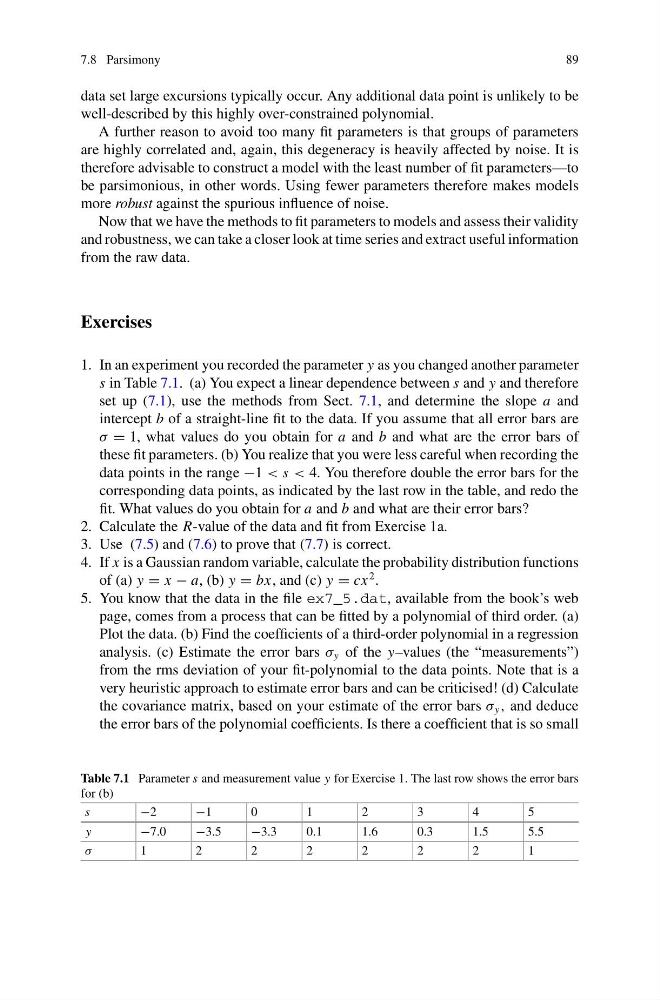
1. In an experiment you recorded the parameter y as you changed another parameter
s in Table 7.1. (a) You expect a linear dependence between s and y and therefore
set up (7.1), use the methods from Sect. 7.1, and determine the slope a and
intercept b of a straight-line fit to the data. If you assume that all error bars are
σ = 1, what values do you obtain for a and b and what are the error bars of
these fit parameters. (b) You realize that you were less careful when recording the
data points in the range −1 < s < 4. You therefore double the error bars for the
corresponding data points, as indicated by the last row in the table, and redo the
fit. What values do you obtain for a and b and what are their error bars?
2. Calculate the R-value of the data and fit from Exercise 1a.
3. Use (7.5) and (7.6) to prove that (7.7) is correct.
4. If x is a Gaussian random variable, calculate the probability distribution functions
of (a) y = x − a, (b) y = bx, and (c) y = cx
2 .
5. You know that the data in the file ex7_5.dat, available from the book’s web
page, comes from a process that can be fitted by a polynomial of third order. (a)
Plot the data. (b) Find the coefficients of a third-order polynomial in a regression
analysis. (c) Estimate the error bars σ y of the y–values (the “measurements”)
from the rms deviation of your fit-polynomial to the data points. Note that is a
very heuristic approach to estimate error bars and can be criticised! (d) Calculate
the covariance matrix, based on your estimate of the error bars σ y , and deduce
the error bars of the polynomial coefficients. Is there a coefficient that is so small
Table 7.1 Parameter s and measurement value y for Exercise 1. The last row shows the error bars
for (b)
s
−2
−1
0
1
2
3
4
5
y
−7.0
−3.5
−3.3
0.1
1.6
0.3
1.5
5.5
σ
1
2
2
2
2
2
2
1
89
data set large excursions typically occur. Any additional data point is unlikely to be
well-described by this highly over-constrained polynomial.
A further reason to avoid too many fit parameters is that groups of parameters
are highly correlated and, again, this degeneracy is heavily affected by noise. It is
therefore advisable to construct a model with the least number of fit parameters—to
be parsimonious, in other words. Using fewer parameters therefore makes models
more robust against the spurious influence of noise.
Now that we have the methods to fit parameters to models and assess their validity
and robustness, we can take a closer look at time series and extract useful information
from the raw data.
Exercises
1. In an experiment you recorded the parameter y as you changed another parameter
s in Table 7.1. (a) You expect a linear dependence between s and y and therefore
set up (7.1), use the methods from Sect. 7.1, and determine the slope a and
intercept b of a straight-line fit to the data. If you assume that all error bars are
σ = 1, what values do you obtain for a and b and what are the error bars of
these fit parameters. (b) You realize that you were less careful when recording the
data points in the range −1 < s < 4. You therefore double the error bars for the
corresponding data points, as indicated by the last row in the table, and redo the
fit. What values do you obtain for a and b and what are their error bars?
2. Calculate the R-value of the data and fit from Exercise 1a.
3. Use (7.5) and (7.6) to prove that (7.7) is correct.
4. If x is a Gaussian random variable, calculate the probability distribution functions
of (a) y = x − a, (b) y = bx, and (c) y = cx
2 .
5. You know that the data in the file ex7_5.dat, available from the book’s web
page, comes from a process that can be fitted by a polynomial of third order. (a)
Plot the data. (b) Find the coefficients of a third-order polynomial in a regression
analysis. (c) Estimate the error bars σ y of the y–values (the “measurements”)
from the rms deviation of your fit-polynomial to the data points. Note that is a
very heuristic approach to estimate error bars and can be criticised! (d) Calculate
the covariance matrix, based on your estimate of the error bars σ y , and deduce
the error bars of the polynomial coefficients. Is there a coefficient that is so small
Table 7.1 Parameter s and measurement value y for Exercise 1. The last row shows the error bars
for (b)
s
−2
−1
0
1
2
3
4
5
y
−7.0
−3.5
−3.3
0.1
1.6
0.3
1.5
5.5
σ
1
2
2
2
2
2
2
1