

7.7 F-Test
87
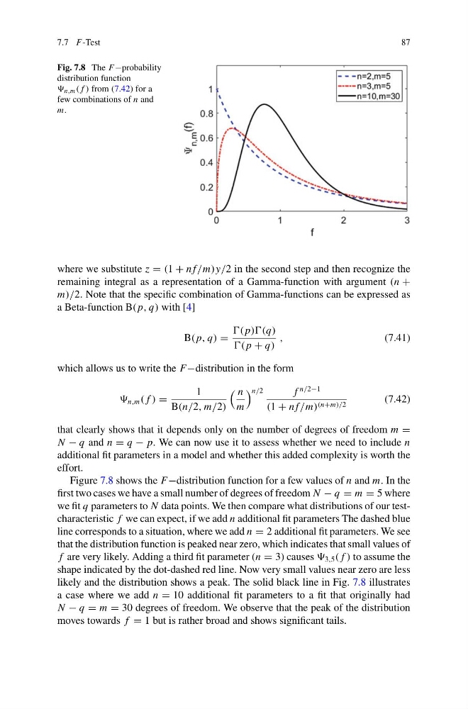
Fig. 7.8 The F−probability
distribution function
n,m ( f ) from (7.42) for a
few combinations of n and
m.
where we substitute z = (1 + n f/m)y/2 in the second step and then recognize the
remaining integral as a representation of a Gamma-function with argument (n +
m)/2. Note that the specific combination of Gamma-functions can be expressed as
a Beta-function B( p, q) with [4]
B( p, q) =
( p))(q)
( p + q)
,
(7.41)
which allows us to write the F−distribution in the form
n,m ( f ) =
1
B(n/2, m/2)
n
m
n/2
f
n/2−1
(1 + n f/m) (n+m)/2
(7.42)
that clearly shows that it depends only on the number of degrees of freedom m =
N − q and n = q − p. We can now use it to assess whether we need to include n
additional fit parameters in a model and whether this added complexity is worth the
effort.
Figure 7.8 shows the F−distribution function for a few values of n and m. In the
first two cases we have a small number of degrees of freedom N − q = m = 5 where
we fit q parameters to N data points. We then compare what distributions of our testcharacteristic f we can expect, if we add n additional fit parameters The dashed blue
line corresponds to a situation, where we add n = 2 additional fit parameters. We see
that the distribution function is peaked near zero, which indicates that small values of
f are very likely. Adding a third fit parameter (n = 3) causes 3,5 ( f ) to assume the
shape indicated by the dot-dashed red line. Now very small values near zero are less
likely and the distribution shows a peak. The solid black line in Fig. 7.8 illustrates
a case where we add n = 10 additional fit parameters to a fit that originally had
N − q = m = 30 degrees of freedom. We observe that the peak of the distribution
moves towards f = 1 but is rather broad and shows significant tails.
87
Fig. 7.8 The F−probability
distribution function
n,m ( f ) from (7.42) for a
few combinations of n and
m.
where we substitute z = (1 + n f/m)y/2 in the second step and then recognize the
remaining integral as a representation of a Gamma-function with argument (n +
m)/2. Note that the specific combination of Gamma-functions can be expressed as
a Beta-function B( p, q) with [4]
B( p, q) =
( p))(q)
( p + q)
,
(7.41)
which allows us to write the F−distribution in the form
n,m ( f ) =
1
B(n/2, m/2)
n
m
n/2
f
n/2−1
(1 + n f/m) (n+m)/2
(7.42)
that clearly shows that it depends only on the number of degrees of freedom m =
N − q and n = q − p. We can now use it to assess whether we need to include n
additional fit parameters in a model and whether this added complexity is worth the
effort.
Figure 7.8 shows the F−distribution function for a few values of n and m. In the
first two cases we have a small number of degrees of freedom N − q = m = 5 where
we fit q parameters to N data points. We then compare what distributions of our testcharacteristic f we can expect, if we add n additional fit parameters The dashed blue
line corresponds to a situation, where we add n = 2 additional fit parameters. We see
that the distribution function is peaked near zero, which indicates that small values of
f are very likely. Adding a third fit parameter (n = 3) causes 3,5 ( f ) to assume the
shape indicated by the dot-dashed red line. Now very small values near zero are less
likely and the distribution shows a peak. The solid black line in Fig. 7.8 illustrates
a case where we add n = 10 additional fit parameters to a fit that originally had
N − q = m = 30 degrees of freedom. We observe that the peak of the distribution
moves towards f = 1 but is rather broad and shows significant tails.