

76
7 Regression Models and Hypothesis Testing
The above manipulations allow us to calculate the fit parameters and their error
bars, but we still do not know how reliable the calculations are, because we could
have a small χ
2 and just had misjudged the initial measurement errors σ i . Therefore
we will first introduce a parameter R
2 that characterizes how well the fitted model
actually explains the observed data y i and then calculate the distribution of χ
2 we
can expect and can judge how likely the obtained χ
2 actually is.
7.3 Goodness-of-Fit R 2
The goodness-of-fit parameter R
2
= SSE/SST compares the spread of the measurement values y i , the total sum of squares (SST), around their mean ¯
y
SST =
n
i=1
(y i − ¯
y)
2
with
¯
y =
1
n
n
i=1
y i
(7.12)
to the explained sum of squares (SSE), defined as the spread of the values ˆ
y i predicted
by the fitted model, to the mean ¯
y
SSE =
n
i=1
( ˆ
y i − ¯
y)
2
with
ˆ
y i =
i
A i j x j .
(7.13)
Here ˆ
y i are the values estimated with the model A i j and the fit parameters x j . R
2 thus
characterizes how well the fitted model can explain the variation around the mean ¯
y.
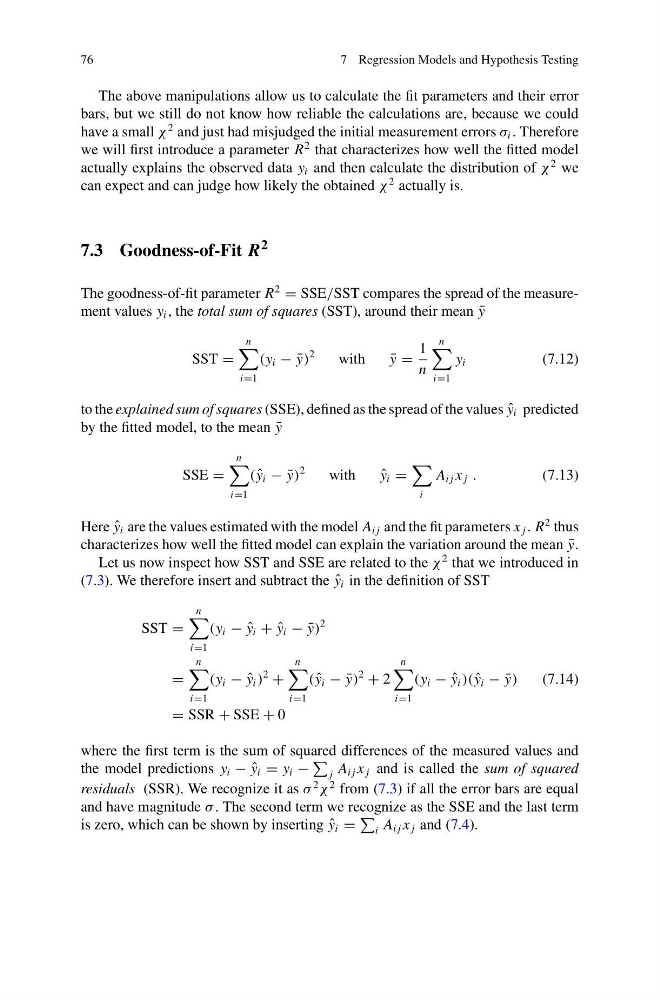
Let us now inspect how SST and SSE are related to the χ
2 that we introduced in
(7.3). We therefore insert and subtract the ˆ
y i in the definition of SST
SST =
n
i=1
(y i − ˆ
y i + ˆ
y i − ¯
y)
2
=
n
i=1
(y i − ˆ
y i )
2
+
n
i=1
( ˆ
y i − ¯
y)
2
+ 2
n
i=1
(y i − ˆ
y i )( ˆ
y i − ¯
y)
(7.14)
= SSR + SSE + 0
where the first term is the sum of squared differences of the measured values and
the model predictions y i − ˆ
y i = y i −
j A i j x j and is called the sum of squared
residuals (SSR). We recognize it as σ
2
χ
2 from (7.3) if all the error bars are equal
and have magnitude σ . The second term we recognize as the SSE and the last term
is zero, which can be shown by inserting ˆ
y i =
i A i j x j and (7.4).
7 Regression Models and Hypothesis Testing
The above manipulations allow us to calculate the fit parameters and their error
bars, but we still do not know how reliable the calculations are, because we could
have a small χ
2 and just had misjudged the initial measurement errors σ i . Therefore
we will first introduce a parameter R
2 that characterizes how well the fitted model
actually explains the observed data y i and then calculate the distribution of χ
2 we
can expect and can judge how likely the obtained χ
2 actually is.
7.3 Goodness-of-Fit R 2
The goodness-of-fit parameter R
2
= SSE/SST compares the spread of the measurement values y i , the total sum of squares (SST), around their mean ¯
y
SST =
n
i=1
(y i − ¯
y)
2
with
¯
y =
1
n
n
i=1
y i
(7.12)
to the explained sum of squares (SSE), defined as the spread of the values ˆ
y i predicted
by the fitted model, to the mean ¯
y
SSE =
n
i=1
( ˆ
y i − ¯
y)
2
with
ˆ
y i =
i
A i j x j .
(7.13)
Here ˆ
y i are the values estimated with the model A i j and the fit parameters x j . R
2 thus
characterizes how well the fitted model can explain the variation around the mean ¯
y.
Let us now inspect how SST and SSE are related to the χ
2 that we introduced in
(7.3). We therefore insert and subtract the ˆ
y i in the definition of SST
SST =
n
i=1
(y i − ˆ
y i + ˆ
y i − ¯
y)
2
=
n
i=1
(y i − ˆ
y i )
2
+
n
i=1
( ˆ
y i − ¯
y)
2
+ 2
n
i=1
(y i − ˆ
y i )( ˆ
y i − ¯
y)
(7.14)
= SSR + SSE + 0
where the first term is the sum of squared differences of the measured values and
the model predictions y i − ˆ
y i = y i −
j A i j x j and is called the sum of squared
residuals (SSR). We recognize it as σ
2
χ
2 from (7.3) if all the error bars are equal
and have magnitude σ . The second term we recognize as the SSE and the last term
is zero, which can be shown by inserting ˆ
y i =
i A i j x j and (7.4).