

7.2 Examples
75
x n+1
˙
x n+1
=
cos(ωωt) (1/ω) sin(ωωt)
−ω sin(ωωt)
cos(ωωt)
x n
˙
x n
.
(7.8)
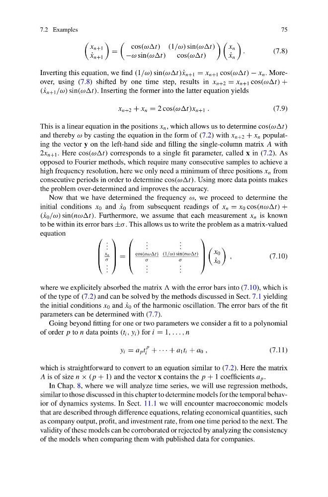
Inverting this equation, we find (1/ω) sin(ωωt) ˙
x n+1 = x n+1 cos(ωωt) − x n . Moreover, using (7.8) shifted by one time step, results in x n+2 = x n+1 cos(ωωt) +
( ˙
x n+1 /ω) sin(ωωt). Inserting the former into the latter equation yields
x n+2 + x n = 2 cos(ωωt)x n+1 .
(7.9)
This is a linear equation in the positions x n , which allows us to determine cos(ωωt)
and thereby ω by casting the equation in the form of (7.2) with x n+2 + x n populating the vector y on the left-hand side and filling the single-column matrix A with
2x n+1 . Here cos(ωωt) corresponds to a single fit parameter, called x in (7.2). As
opposed to Fourier methods, which require many consecutive samples to achieve a
high frequency resolution, here we only need a minimum of three positions x n from
consecutive periods in order to determine cos(ωωt). Using more data points makes
the problem over-determined and improves the accuracy.
Now that we have determined the frequency ω, we proceed to determine the
initial conditions x 0 and ˙
x 0 from subsequent readings of x n = x 0 cos(nωωt) +
( ˙
x 0 /ω) sin(nωωt). Furthermore, we assume that each measurement x n is known
to be within its error bars ±σ . This allows us to write the problem as a matrix-valued
equation
⎛
⎜
⎜
⎝
. . .
x n
σ
. . .
⎞
⎟
⎟
⎠ =
⎛
⎜
⎜
⎝
. . .
. . .
cos(nωωt)
σ
(1/ω) sin(nωωt)
σ
. . .
. . .
⎞
⎟
⎟
⎠
x 0
˙
x 0
,
(7.10)
where we explicitely absorbed the matrix with the error bars into (7.10), which is
of the type of (7.2) and can be solved by the methods discussed in Sect. 7.1 yielding
the initial conditions x 0 and ˙
x 0 of the harmonic oscillation. The error bars of the fit
parameters can be determined with (7.7).
Going beyond fitting for one or two parameters we consider a fit to a polynomial
of order p to n data points (t i , y i ) for i = 1, . . . , n
y i = a p t
p
i + · · · + a 1 t i + a 0 ,
(7.11)
which is straightforward to convert to an equation similar to (7.2). Here the matrix
A is of size n × ( p + 1) and the vector x contains the p + 1 coefficients a p .
In Chap. 8, where we will analyze time series, we will use regression methods,
similar to those discussed in this chapter to determine models for the temporal behavior of dynamics systems. In Sect. 11.1 we will encounter macroeconomic models
that are described through difference equations, relating economical quantities, such
as company output, profit, and investment rate, from one time period to the next. The
validity of these models can be corroborated or rejected by analyzing the consistency
of the models when comparing them with published data for companies.
75
x n+1
˙
x n+1
=
cos(ωωt) (1/ω) sin(ωωt)
−ω sin(ωωt)
cos(ωωt)
x n
˙
x n
.
(7.8)
Inverting this equation, we find (1/ω) sin(ωωt) ˙
x n+1 = x n+1 cos(ωωt) − x n . Moreover, using (7.8) shifted by one time step, results in x n+2 = x n+1 cos(ωωt) +
( ˙
x n+1 /ω) sin(ωωt). Inserting the former into the latter equation yields
x n+2 + x n = 2 cos(ωωt)x n+1 .
(7.9)
This is a linear equation in the positions x n , which allows us to determine cos(ωωt)
and thereby ω by casting the equation in the form of (7.2) with x n+2 + x n populating the vector y on the left-hand side and filling the single-column matrix A with
2x n+1 . Here cos(ωωt) corresponds to a single fit parameter, called x in (7.2). As
opposed to Fourier methods, which require many consecutive samples to achieve a
high frequency resolution, here we only need a minimum of three positions x n from
consecutive periods in order to determine cos(ωωt). Using more data points makes
the problem over-determined and improves the accuracy.
Now that we have determined the frequency ω, we proceed to determine the
initial conditions x 0 and ˙
x 0 from subsequent readings of x n = x 0 cos(nωωt) +
( ˙
x 0 /ω) sin(nωωt). Furthermore, we assume that each measurement x n is known
to be within its error bars ±σ . This allows us to write the problem as a matrix-valued
equation
⎛
⎜
⎜
⎝
. . .
x n
σ
. . .
⎞
⎟
⎟
⎠ =
⎛
⎜
⎜
⎝
. . .
. . .
cos(nωωt)
σ
(1/ω) sin(nωωt)
σ
. . .
. . .
⎞
⎟
⎟
⎠
x 0
˙
x 0
,
(7.10)
where we explicitely absorbed the matrix with the error bars into (7.10), which is
of the type of (7.2) and can be solved by the methods discussed in Sect. 7.1 yielding
the initial conditions x 0 and ˙
x 0 of the harmonic oscillation. The error bars of the fit
parameters can be determined with (7.7).
Going beyond fitting for one or two parameters we consider a fit to a polynomial
of order p to n data points (t i , y i ) for i = 1, . . . , n
y i = a p t
p
i + · · · + a 1 t i + a 0 ,
(7.11)
which is straightforward to convert to an equation similar to (7.2). Here the matrix
A is of size n × ( p + 1) and the vector x contains the p + 1 coefficients a p .
In Chap. 8, where we will analyze time series, we will use regression methods,
similar to those discussed in this chapter to determine models for the temporal behavior of dynamics systems. In Sect. 11.1 we will encounter macroeconomic models
that are described through difference equations, relating economical quantities, such
as company output, profit, and investment rate, from one time period to the next. The
validity of these models can be corroborated or rejected by analyzing the consistency
of the models when comparing them with published data for companies.