

74
7 Regression Models and Hypothesis Testing
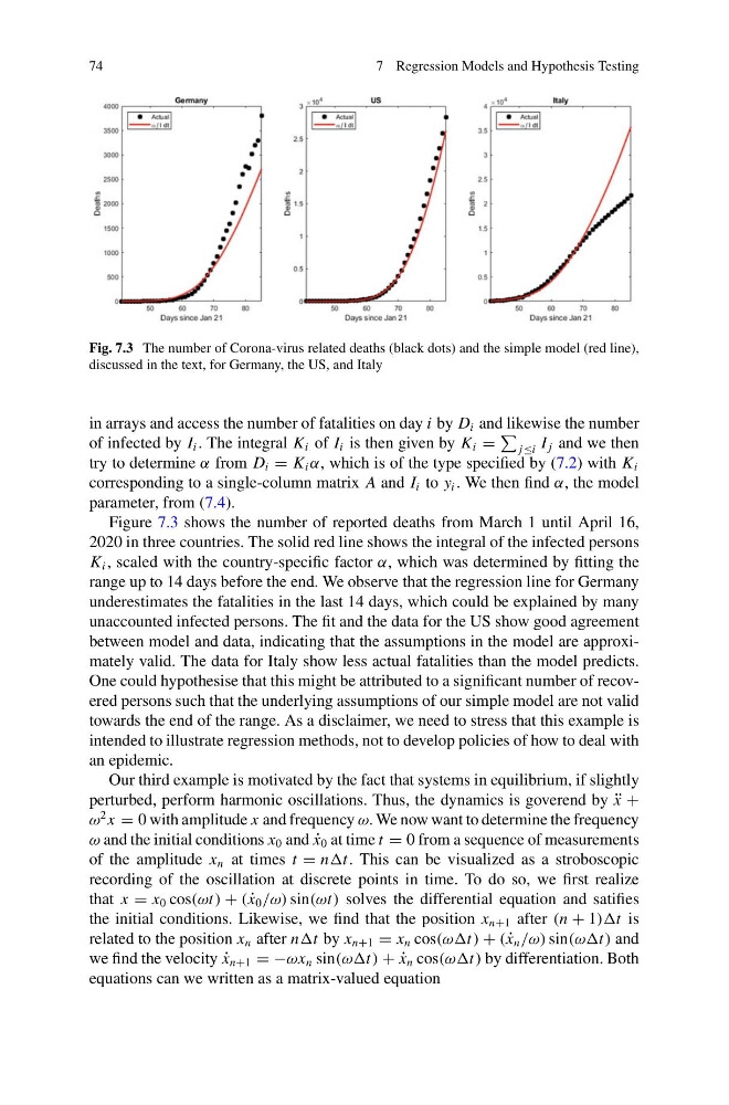
Fig. 7.3 The number of Corona-virus related deaths (black dots) and the simple model (red line),
discussed in the text, for Germany, the US, and Italy
in arrays and access the number of fatalities on day i by D i and likewise the number
of infected by I i . The integral K i of I i is then given by K i =
j≤i I j and we then
try to determine α from D i = K i α, which is of the type specified by (7.2) with K i
corresponding to a single-column matrix A and I i to y i . We then find α, the model
parameter, from (7.4).
Figure 7.3 shows the number of reported deaths from March 1 until April 16,
2020 in three countries. The solid red line shows the integral of the infected persons
K i , scaled with the country-specific factor α, which was determined by fitting the
range up to 14 days before the end. We observe that the regression line for Germany
underestimates the fatalities in the last 14 days, which could be explained by many
unaccounted infected persons. The fit and the data for the US show good agreement
between model and data, indicating that the assumptions in the model are approximately valid. The data for Italy show less actual fatalities than the model predicts.
One could hypothesise that this might be attributed to a significant number of recovered persons such that the underlying assumptions of our simple model are not valid
towards the end of the range. As a disclaimer, we need to stress that this example is
intended to illustrate regression methods, not to develop policies of how to deal with
an epidemic.
Our third example is motivated by the fact that systems in equilibrium, if slightly
perturbed, perform harmonic oscillations. Thus, the dynamics is goverend by ¨
x +
ω
2 x = 0 with amplitude x and frequency ω. We now want to determine the frequency
ω and the initial conditions x 0 and ˙
x 0 at time t = 0 from a sequence of measurements
of the amplitude x n at times t = nt. This can be visualized as a stroboscopic
recording of the oscillation at discrete points in time. To do so, we first realize
that x = x 0 cos(ωt) + ( ˙
x 0 /ω) sin(ωt) solves the differential equation and satifies
the initial conditions. Likewise, we find that the position x n+1 after (n + 1))t is
related to the position x n after nt by x n+1 = x n cos(ωωt) + ( ˙
x n /ω) sin(ωωt) and
we find the velocity ˙
x n+1 = −ωx n sin(ωt) + ˙
x n cos(ωωt) by differentiation. Both
equations can we written as a matrix-valued equation
7 Regression Models and Hypothesis Testing
Fig. 7.3 The number of Corona-virus related deaths (black dots) and the simple model (red line),
discussed in the text, for Germany, the US, and Italy
in arrays and access the number of fatalities on day i by D i and likewise the number
of infected by I i . The integral K i of I i is then given by K i =
j≤i I j and we then
try to determine α from D i = K i α, which is of the type specified by (7.2) with K i
corresponding to a single-column matrix A and I i to y i . We then find α, the model
parameter, from (7.4).
Figure 7.3 shows the number of reported deaths from March 1 until April 16,
2020 in three countries. The solid red line shows the integral of the infected persons
K i , scaled with the country-specific factor α, which was determined by fitting the
range up to 14 days before the end. We observe that the regression line for Germany
underestimates the fatalities in the last 14 days, which could be explained by many
unaccounted infected persons. The fit and the data for the US show good agreement
between model and data, indicating that the assumptions in the model are approximately valid. The data for Italy show less actual fatalities than the model predicts.
One could hypothesise that this might be attributed to a significant number of recovered persons such that the underlying assumptions of our simple model are not valid
towards the end of the range. As a disclaimer, we need to stress that this example is
intended to illustrate regression methods, not to develop policies of how to deal with
an epidemic.
Our third example is motivated by the fact that systems in equilibrium, if slightly
perturbed, perform harmonic oscillations. Thus, the dynamics is goverend by ¨
x +
ω
2 x = 0 with amplitude x and frequency ω. We now want to determine the frequency
ω and the initial conditions x 0 and ˙
x 0 at time t = 0 from a sequence of measurements
of the amplitude x n at times t = nt. This can be visualized as a stroboscopic
recording of the oscillation at discrete points in time. To do so, we first realize
that x = x 0 cos(ωt) + ( ˙
x 0 /ω) sin(ωt) solves the differential equation and satifies
the initial conditions. Likewise, we find that the position x n+1 after (n + 1))t is
related to the position x n after nt by x n+1 = x n cos(ωωt) + ( ˙
x n /ω) sin(ωωt) and
we find the velocity ˙
x n+1 = −ωx n sin(ωt) + ˙
x n cos(ωωt) by differentiation. Both
equations can we written as a matrix-valued equation