

7.2 Examples
73
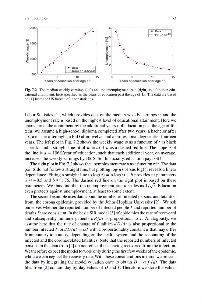
Fig. 7.2 The median weekly earnings (left) and the unemployment rate (right) as a function educational attainment, here specified as the years of education past the age of 15. The data are based
on [1] from the US bureau of labor statistics
Labor Statistics [1], which provides data on the median weekly earnings w and the
unemployment rate u based on the highest level of educational attainment. Here we
characterize the attainment by the additional years t of education past the age of fifteen; we assume a high-school diploma completed after two years, a bachelor after
six, a master after eight, a PhD after twelve, and a professional degree after fourteen
years. The left plot in Fig. 7.2 shows the weekly wage w as a function of t as black
asterisks and a straight-line fit of w = at + b as a dashed red line. The slope a of
the line is a = 106 $/year of education, such that each additional year, on average,
increases the weekly earnings by 106 $. So, financially, education pays off!
The right plot in Fig. 7.2 shows the unemployment rate u as a function of t. The data
points do not follow a straight line, but plotting log(u) versus log(t) reveals a linear
dependence. Fitting a straight line to log(u) = a log(t) + b provides fit parameters
a ≈ −0.5 and b ≈ 1.76. The dashed red line on the right plot is based on these
parameters. We thus find that the unemployment rate u scales as 1/
√
t. Education
even protects against unemployment, at least to some extent.
The second example uses data about the number of infected persons and fatalities
from the corona epidemic, provided by the Johns-Hopkins University [2]. We ask
ourselves whether the reported number of infected people I and reported number of
deaths D are consistent. In the basic SIR model [3] of epidemics the rate of recovered
and subsequently immune patients d R/dt is proportional to I . Analogously, we
assume here that the rate of change of fatalities d D/dt is also proportional to the
number infected I , or d D/dt = α I with a proportionality constant α that may differ
from country to country, depending on the health system and the accounting of the
infected and the corona-related fatalities. Note that the reported numbers of infected
persons in the data from [2] do not reflect those having recovered from the infection.
We therefore expect the model to work only during the first few weeks of the epidemic,
while we can neglect the recovery rate. With these considerations in mind we process
the data by integrating the model equation once to obtain D = α
I dt. The data
files from [2] contain day-by-day values of D and I . Therefore we store the values
73
Fig. 7.2 The median weekly earnings (left) and the unemployment rate (right) as a function educational attainment, here specified as the years of education past the age of 15. The data are based
on [1] from the US bureau of labor statistics
Labor Statistics [1], which provides data on the median weekly earnings w and the
unemployment rate u based on the highest level of educational attainment. Here we
characterize the attainment by the additional years t of education past the age of fifteen; we assume a high-school diploma completed after two years, a bachelor after
six, a master after eight, a PhD after twelve, and a professional degree after fourteen
years. The left plot in Fig. 7.2 shows the weekly wage w as a function of t as black
asterisks and a straight-line fit of w = at + b as a dashed red line. The slope a of
the line is a = 106 $/year of education, such that each additional year, on average,
increases the weekly earnings by 106 $. So, financially, education pays off!
The right plot in Fig. 7.2 shows the unemployment rate u as a function of t. The data
points do not follow a straight line, but plotting log(u) versus log(t) reveals a linear
dependence. Fitting a straight line to log(u) = a log(t) + b provides fit parameters
a ≈ −0.5 and b ≈ 1.76. The dashed red line on the right plot is based on these
parameters. We thus find that the unemployment rate u scales as 1/
√
t. Education
even protects against unemployment, at least to some extent.
The second example uses data about the number of infected persons and fatalities
from the corona epidemic, provided by the Johns-Hopkins University [2]. We ask
ourselves whether the reported number of infected people I and reported number of
deaths D are consistent. In the basic SIR model [3] of epidemics the rate of recovered
and subsequently immune patients d R/dt is proportional to I . Analogously, we
assume here that the rate of change of fatalities d D/dt is also proportional to the
number infected I , or d D/dt = α I with a proportionality constant α that may differ
from country to country, depending on the health system and the accounting of the
infected and the corona-related fatalities. Note that the reported numbers of infected
persons in the data from [2] do not reflect those having recovered from the infection.
We therefore expect the model to work only during the first few weeks of the epidemic,
while we can neglect the recovery rate. With these considerations in mind we process
the data by integrating the model equation once to obtain D = α
I dt. The data
files from [2] contain day-by-day values of D and I . Therefore we store the values