

7.3 Goodness-of-Fit R 2
77
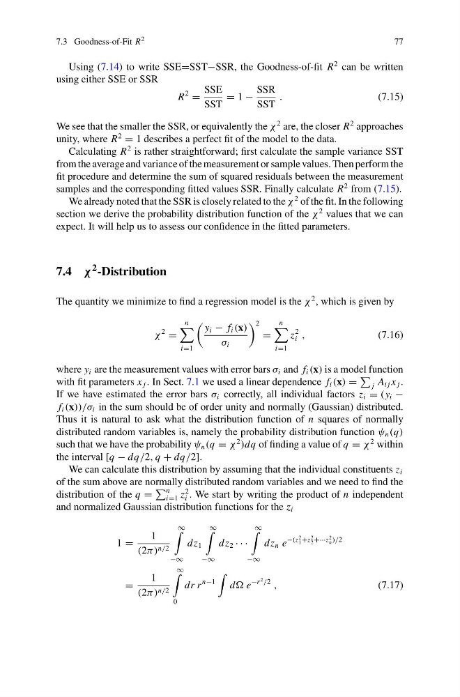
Using (7.14) to write SSE=SST−SSR, the Goodness-of-fit R
2 can be written
using either SSE or SSR
R
2
=
SSE
SST
= 1 −
SSR
SST
.
(7.15)
We see that the smaller the SSR, or equivalently the χ
2 are, the closer R
2 approaches
unity, where R
2
= 1 describes a perfect fit of the model to the data.
Calculating R
2 is rather straightforward; first calculate the sample variance SST
from the average and variance of the measurement or sample values. Then perform the
fit procedure and determine the sum of squared residuals between the measurement
samples and the corresponding fitted values SSR. Finally calculate R
2 from (7.15).
We already noted that the SSR is closely related to the χ
2 of the fit. In the following
section we derive the probability distribution function of the χ
2 values that we can
expect. It will help us to assess our confidence in the fitted parameters.
7.4 χ 2 -Distribution
The quantity we minimize to find a regression model is the χ
2 , which is given by
χ
2
=
n
i=1
y i − f i (x)
σ i
2
=
n
i=1
z
2
i ,
(7.16)
where y i are the measurement values with error bars σ i and f i (x) is a model function
with fit parameters x j . In Sect. 7.1 we used a linear dependence f i (x) =
j A i j x j .
If we have estimated the error bars σ i correctly, all individual factors z i = (y i −
f i (x))/σ i in the sum should be of order unity and normally (Gaussian) distributed.
Thus it is natural to ask what the distribution function of n squares of normally
distributed random variables is, namely the probability distribution function ψ n (q)
such that we have the probability ψ n (q = χ
2
)dq of finding a value of q = χ
2 within
the interval [q − dq/2, q + dq/2].
We can calculate this distribution by assuming that the individual constituents z i
of the sum above are normally distributed random variables and we need to find the
distribution of the q =
n
i=1 z
2
i . We start by writing the product of n independent
and normalized Gaussian distribution functions for the z i
1 =
1
(2π) n/2
∞
−∞
dz 1
∞
−∞
dz 2 · · ·
∞
−∞
dz n e
−(z
2
1 +z
2
2 +···z
2
n )/2
=
1
(2π) n/2
∞
0
dr r
n−1
d e
−r
2 /2
,
(7.17)
77
Using (7.14) to write SSE=SST−SSR, the Goodness-of-fit R
2 can be written
using either SSE or SSR
R
2
=
SSE
SST
= 1 −
SSR
SST
.
(7.15)
We see that the smaller the SSR, or equivalently the χ
2 are, the closer R
2 approaches
unity, where R
2
= 1 describes a perfect fit of the model to the data.
Calculating R
2 is rather straightforward; first calculate the sample variance SST
from the average and variance of the measurement or sample values. Then perform the
fit procedure and determine the sum of squared residuals between the measurement
samples and the corresponding fitted values SSR. Finally calculate R
2 from (7.15).
We already noted that the SSR is closely related to the χ
2 of the fit. In the following
section we derive the probability distribution function of the χ
2 values that we can
expect. It will help us to assess our confidence in the fitted parameters.
7.4 χ 2 -Distribution
The quantity we minimize to find a regression model is the χ
2 , which is given by
χ
2
=
n
i=1
y i − f i (x)
σ i
2
=
n
i=1
z
2
i ,
(7.16)
where y i are the measurement values with error bars σ i and f i (x) is a model function
with fit parameters x j . In Sect. 7.1 we used a linear dependence f i (x) =
j A i j x j .
If we have estimated the error bars σ i correctly, all individual factors z i = (y i −
f i (x))/σ i in the sum should be of order unity and normally (Gaussian) distributed.
Thus it is natural to ask what the distribution function of n squares of normally
distributed random variables is, namely the probability distribution function ψ n (q)
such that we have the probability ψ n (q = χ
2
)dq of finding a value of q = χ
2 within
the interval [q − dq/2, q + dq/2].
We can calculate this distribution by assuming that the individual constituents z i
of the sum above are normally distributed random variables and we need to find the
distribution of the q =
n
i=1 z
2
i . We start by writing the product of n independent
and normalized Gaussian distribution functions for the z i
1 =
1
(2π) n/2
∞
−∞
dz 1
∞
−∞
dz 2 · · ·
∞
−∞
dz n e
−(z
2
1 +z
2
2 +···z
2
n )/2
=
1
(2π) n/2
∞
0
dr r
n−1
d e
−r
2 /2
,
(7.17)