

4.5 Master and Fokker-Planck Equations
39
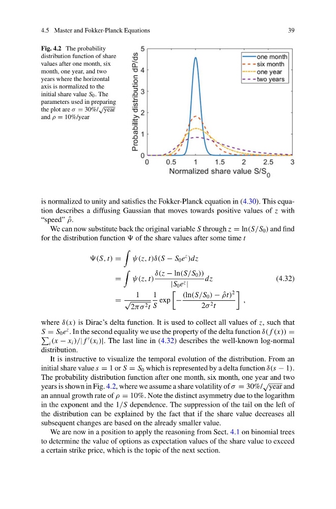
Fig. 4.2 The probability
distribution function of share
values after one month, six
month, one year, and two
years where the horizontal
axis is normalized to the
initial share value S 0 . The
parameters used in preparing
the plot are σ = 30%/
√ year
and ρ = 10%/year
is normalized to unity and satisfies the Fokker-Planck equation in (4.30). This equation describes a diffusing Gaussian that moves towards positive values of z with
“speed” ˆ
ρ.
We can now substitute back the original variable S through z = ln(S/S 0 ) and find
for the distribution function of the share values after some time t
(S, t) =
ψ(z, t)δ(S − S 0 e
z
)dz
=
ψ(z, t)
δ(z − ln(S/S 0 ))
|S 0 e z |
dz
(4.32)
=
1
√
2πσ 2 t
1
S
exp
−
(ln(S/S 0 ) − ˆ
ρt)
2
2σ 2 t
,
where δ(x) is Dirac’s delta function. It is used to collect all values of z, such that
S = S 0 e
z . In the second equality we use the property of the delta function δ( f (x)) =
i (x − x i )/| f
(x i )|. The last line in (4.32) describes the well-known log-normal
distribution.
It is instructive to visualize the temporal evolution of the distribution. From an
initial share value s = 1 or S = S 0 which is represented by a delta function δ(s − 1).
The probability distribution function after one month, six month, one year and two
years is shown in Fig. 4.2, where we assume a share volatility of σ = 30%/
√ year and
an annual growth rate of ρ = 10%. Note the distinct asymmetry due to the logarithm
in the exponent and the 1/S dependence. The suppression of the tail on the left of
the distribution can be explained by the fact that if the share value decreases all
subsequent changes are based on the already smaller value.
We are now in a position to apply the reasoning from Sect. 4.1 on binomial trees
to determine the value of options as expectation values of the share value to exceed
a certain strike price, which is the topic of the next section.
39
Fig. 4.2 The probability
distribution function of share
values after one month, six
month, one year, and two
years where the horizontal
axis is normalized to the
initial share value S 0 . The
parameters used in preparing
the plot are σ = 30%/
√ year
and ρ = 10%/year
is normalized to unity and satisfies the Fokker-Planck equation in (4.30). This equation describes a diffusing Gaussian that moves towards positive values of z with
“speed” ˆ
ρ.
We can now substitute back the original variable S through z = ln(S/S 0 ) and find
for the distribution function of the share values after some time t
(S, t) =
ψ(z, t)δ(S − S 0 e
z
)dz
=
ψ(z, t)
δ(z − ln(S/S 0 ))
|S 0 e z |
dz
(4.32)
=
1
√
2πσ 2 t
1
S
exp
−
(ln(S/S 0 ) − ˆ
ρt)
2
2σ 2 t
,
where δ(x) is Dirac’s delta function. It is used to collect all values of z, such that
S = S 0 e
z . In the second equality we use the property of the delta function δ( f (x)) =
i (x − x i )/| f
(x i )|. The last line in (4.32) describes the well-known log-normal
distribution.
It is instructive to visualize the temporal evolution of the distribution. From an
initial share value s = 1 or S = S 0 which is represented by a delta function δ(s − 1).
The probability distribution function after one month, six month, one year and two
years is shown in Fig. 4.2, where we assume a share volatility of σ = 30%/
√ year and
an annual growth rate of ρ = 10%. Note the distinct asymmetry due to the logarithm
in the exponent and the 1/S dependence. The suppression of the tail on the left of
the distribution can be explained by the fact that if the share value decreases all
subsequent changes are based on the already smaller value.
We are now in a position to apply the reasoning from Sect. 4.1 on binomial trees
to determine the value of options as expectation values of the share value to exceed
a certain strike price, which is the topic of the next section.