

38
4 Stochastic Processes
ψ(z, t + dτ ) = ψ(z, t) +
∂ψ
∂t
dτ .
(4.26)
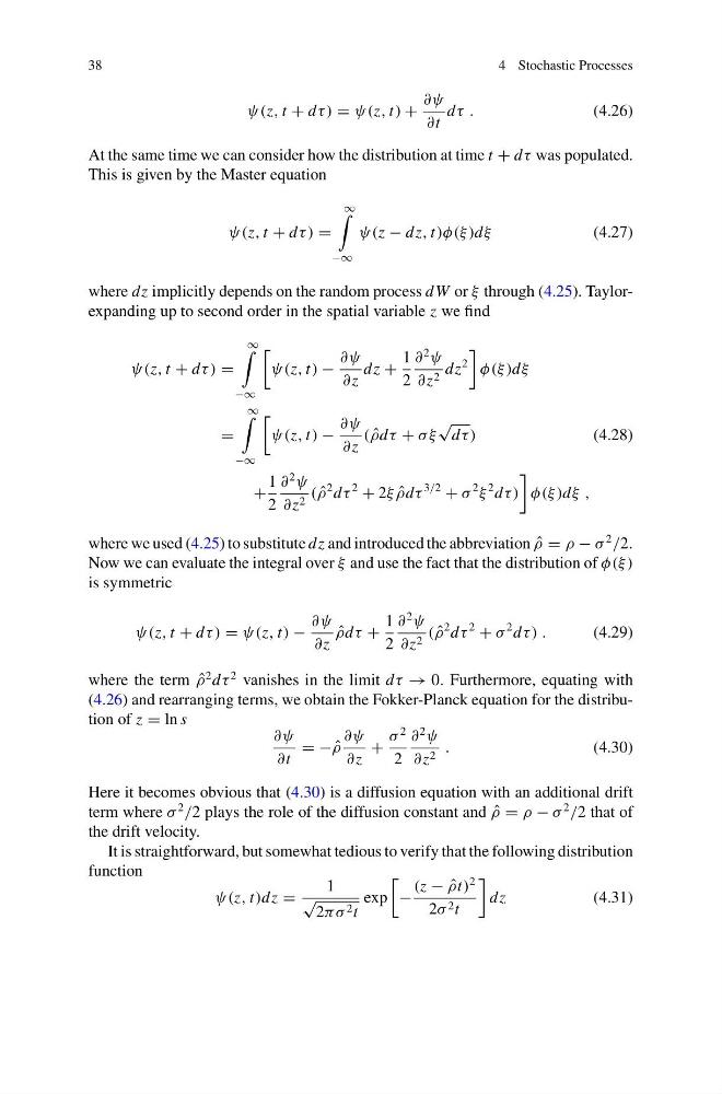
At the same time we can consider how the distribution at time t + dτ was populated.
This is given by the Master equation
ψ(z, t + dτ ) =
∞
−∞
ψ(z − dz, t)φ(ξ )dξ
(4.27)
where dz implicitly depends on the random process dW or ξ through (4.25). Taylorexpanding up to second order in the spatial variable z we find
ψ(z, t + dτ ) =
∞
−∞
ψ(z, t) −
∂ψ
∂z
dz +
1
2
∂
2
ψ
∂z 2 dz
2
φ(ξ )dξ
=
∞
−∞
ψ(z, t) −
∂ψ
∂z
( ˆ
ρdτ + σ ξ
√
dτ )
(4.28)
+
1
2
∂
2
ψ
∂z 2 ( ˆ
ρ
2 dτ
2
+ 2ξ ˆ
ρdτ
3/2
+ σ
2
ξ
2 dτ )
φ(ξ )dξ ,
where we used (4.25) to substitute dz and introduced the abbreviation ˆ
ρ = ρ − σ
2
/2.
Now we can evaluate the integral over ξ and use the fact that the distribution of φ(ξ )
is symmetric
ψ(z, t + dτ ) = ψ(z, t) −
∂ψ
∂z
ˆ
ρdτ +
1
2
∂
2
ψ
∂z 2 ( ˆ
ρ
2 dτ
2
+ σ
2 dτ ) .
(4.29)
where the term ˆ
ρ
2 dτ
2 vanishes in the limit dτ → 0. Furthermore, equating with
(4.26) and rearranging terms, we obtain the Fokker-Planck equation for the distribution of z = ln s
∂ψ
∂t
= − ˆ
ρ
∂ψ
∂z
+
σ
2
2
∂
2
ψ
∂z 2 .
(4.30)
Here it becomes obvious that (4.30) is a diffusion equation with an additional drift
term where σ
2
/2 plays the role of the diffusion constant and ˆ
ρ = ρ − σ
2
/2 that of
the drift velocity.
It is straightforward, but somewhat tedious to verify that the following distribution
function
ψ(z, t)dz =
1
√
2πσ 2 t
exp
−
(z − ˆ
ρt)
2
2σ 2 t
dz
(4.31)
4 Stochastic Processes
ψ(z, t + dτ ) = ψ(z, t) +
∂ψ
∂t
dτ .
(4.26)
At the same time we can consider how the distribution at time t + dτ was populated.
This is given by the Master equation
ψ(z, t + dτ ) =
∞
−∞
ψ(z − dz, t)φ(ξ )dξ
(4.27)
where dz implicitly depends on the random process dW or ξ through (4.25). Taylorexpanding up to second order in the spatial variable z we find
ψ(z, t + dτ ) =
∞
−∞
ψ(z, t) −
∂ψ
∂z
dz +
1
2
∂
2
ψ
∂z 2 dz
2
φ(ξ )dξ
=
∞
−∞
ψ(z, t) −
∂ψ
∂z
( ˆ
ρdτ + σ ξ
√
dτ )
(4.28)
+
1
2
∂
2
ψ
∂z 2 ( ˆ
ρ
2 dτ
2
+ 2ξ ˆ
ρdτ
3/2
+ σ
2
ξ
2 dτ )
φ(ξ )dξ ,
where we used (4.25) to substitute dz and introduced the abbreviation ˆ
ρ = ρ − σ
2
/2.
Now we can evaluate the integral over ξ and use the fact that the distribution of φ(ξ )
is symmetric
ψ(z, t + dτ ) = ψ(z, t) −
∂ψ
∂z
ˆ
ρdτ +
1
2
∂
2
ψ
∂z 2 ( ˆ
ρ
2 dτ
2
+ σ
2 dτ ) .
(4.29)
where the term ˆ
ρ
2 dτ
2 vanishes in the limit dτ → 0. Furthermore, equating with
(4.26) and rearranging terms, we obtain the Fokker-Planck equation for the distribution of z = ln s
∂ψ
∂t
= − ˆ
ρ
∂ψ
∂z
+
σ
2
2
∂
2
ψ
∂z 2 .
(4.30)
Here it becomes obvious that (4.30) is a diffusion equation with an additional drift
term where σ
2
/2 plays the role of the diffusion constant and ˆ
ρ = ρ − σ
2
/2 that of
the drift velocity.
It is straightforward, but somewhat tedious to verify that the following distribution
function
ψ(z, t)dz =
1
√
2πσ 2 t
exp
−
(z − ˆ
ρt)
2
2σ 2 t
dz
(4.31)