

4.4 Stochastic Integrals and Ito’s Lemma
37
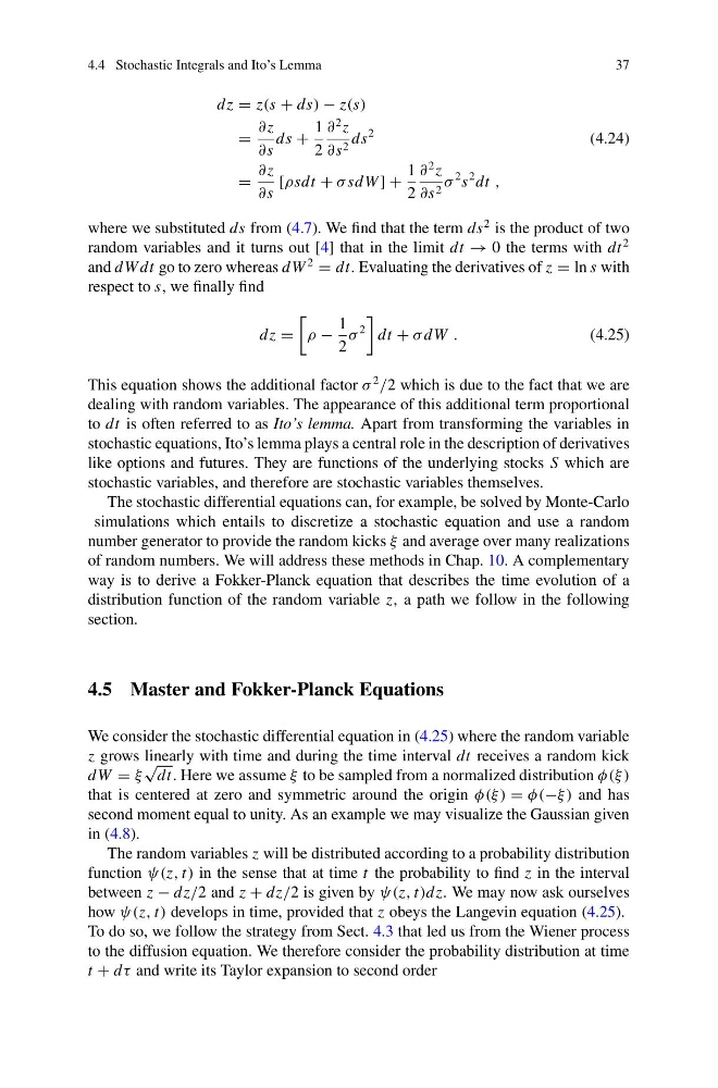
dz = z(s + ds) − z(s)
=
∂z
∂s
ds +
1
2
∂
2 z
∂s 2 ds
2
(4.24)
=
∂z
∂s
[ρsdt + σ sdW ] +
1
2
∂
2 z
∂s 2 σ
2 s
2 dt ,
where we substituted ds from (4.7). We find that the term ds
2 is the product of two
random variables and it turns out [4] that in the limit dt → 0 the terms with dt
2
and dW dt go to zero whereas dW
2
= dt. Evaluating the derivatives of z = ln s with
respect to s, we finally find
dz =
ρ −
1
2
σ
2
dt + σ dW .
(4.25)
This equation shows the additional factor σ
2
/2 which is due to the fact that we are
dealing with random variables. The appearance of this additional term proportional
to dt is often referred to as Ito’s lemma. Apart from transforming the variables in
stochastic equations, Ito’s lemma plays a central role in the description of derivatives
like options and futures. They are functions of the underlying stocks S which are
stochastic variables, and therefore are stochastic variables themselves.
The stochastic differential equations can, for example, be solved by Monte-Carlo
simulations which entails to discretize a stochastic equation and use a random
number generator to provide the random kicks ξ and average over many realizations
of random numbers. We will address these methods in Chap. 10. A complementary
way is to derive a Fokker-Planck equation that describes the time evolution of a
distribution function of the random variable z, a path we follow in the following
section.
4.5 Master and Fokker-Planck Equations
We consider the stochastic differential equation in (4.25) where the random variable
z grows linearly with time and during the time interval dt receives a random kick
dW = ξ
√
dt. Here we assume ξ to be sampled from a normalized distribution φ(ξ )
that is centered at zero and symmetric around the origin φ(ξ ) = φ(−ξ) and has
second moment equal to unity. As an example we may visualize the Gaussian given
in (4.8).
The random variables z will be distributed according to a probability distribution
function ψ(z, t) in the sense that at time t the probability to find z in the interval
between z − dz/2 and z + dz/2 is given by ψ(z, t)dz. We may now ask ourselves
how ψ(z, t) develops in time, provided that z obeys the Langevin equation (4.25).
To do so, we follow the strategy from Sect. 4.3 that led us from the Wiener process
to the diffusion equation. We therefore consider the probability distribution at time
t + dτ and write its Taylor expansion to second order
37
dz = z(s + ds) − z(s)
=
∂z
∂s
ds +
1
2
∂
2 z
∂s 2 ds
2
(4.24)
=
∂z
∂s
[ρsdt + σ sdW ] +
1
2
∂
2 z
∂s 2 σ
2 s
2 dt ,
where we substituted ds from (4.7). We find that the term ds
2 is the product of two
random variables and it turns out [4] that in the limit dt → 0 the terms with dt
2
and dW dt go to zero whereas dW
2
= dt. Evaluating the derivatives of z = ln s with
respect to s, we finally find
dz =
ρ −
1
2
σ
2
dt + σ dW .
(4.25)
This equation shows the additional factor σ
2
/2 which is due to the fact that we are
dealing with random variables. The appearance of this additional term proportional
to dt is often referred to as Ito’s lemma. Apart from transforming the variables in
stochastic equations, Ito’s lemma plays a central role in the description of derivatives
like options and futures. They are functions of the underlying stocks S which are
stochastic variables, and therefore are stochastic variables themselves.
The stochastic differential equations can, for example, be solved by Monte-Carlo
simulations which entails to discretize a stochastic equation and use a random
number generator to provide the random kicks ξ and average over many realizations
of random numbers. We will address these methods in Chap. 10. A complementary
way is to derive a Fokker-Planck equation that describes the time evolution of a
distribution function of the random variable z, a path we follow in the following
section.
4.5 Master and Fokker-Planck Equations
We consider the stochastic differential equation in (4.25) where the random variable
z grows linearly with time and during the time interval dt receives a random kick
dW = ξ
√
dt. Here we assume ξ to be sampled from a normalized distribution φ(ξ )
that is centered at zero and symmetric around the origin φ(ξ ) = φ(−ξ) and has
second moment equal to unity. As an example we may visualize the Gaussian given
in (4.8).
The random variables z will be distributed according to a probability distribution
function ψ(z, t) in the sense that at time t the probability to find z in the interval
between z − dz/2 and z + dz/2 is given by ψ(z, t)dz. We may now ask ourselves
how ψ(z, t) develops in time, provided that z obeys the Langevin equation (4.25).
To do so, we follow the strategy from Sect. 4.3 that led us from the Wiener process
to the diffusion equation. We therefore consider the probability distribution at time
t + dτ and write its Taylor expansion to second order