

36
4 Stochastic Processes
Comparing (4.20) with (4.22), we observe that the first is a (partial) differential
equation that specifies how to find the Laplace operator applied to the potential U.
But we do not want to know U ; we want to know U (x), and (4.22) provides us with
just that information. It determines U directly, albeit at the expense of calculating the
integral over the charge distribution, weighted with an integral kernel, the Green’s
function. The latter has, however, the intuitive interpretation as the potential of a
point charge.
Note that the Green’s functions can be viewed as the response U to a stimulus
ρ where we calculate U with a convolution integral over ρ. This is conceptionally
similar to what happens in electrical filters. They are stimulated by external, possibly
noisy, signals and then remove the noise by, for example, low-pass filtering. The
filter function in these applications assumes the same role as the Green’s function
where the noisy input signal is convoluted with the filter function. Moreover the
propagators in quantum field theory, which mediate the fundamental interactions,
are Green’s functions that are caused by one particle and mediate its stimulus to a
second particle. We will encounter this concept repeatedly in the following chapters.
In the next sections, however, we will address the use of stochastic differential
equations in a financial context.
4.4 Stochastic Integrals and Ito’s Lemma
In (4.7) looms a second specialty of stochastic processes, namely the product of two
random variables s and dW. Both are jumping and this requires some additional
discussion about how to evaluate the product when it appears in an integral, which is
what we need in order to step (4.7) forward in time. There are two commonly used
ways how to handle the products [4], one according to Stratonovich and the other
is due to Ito. The latter is commonly used in finance and the interpretation of the
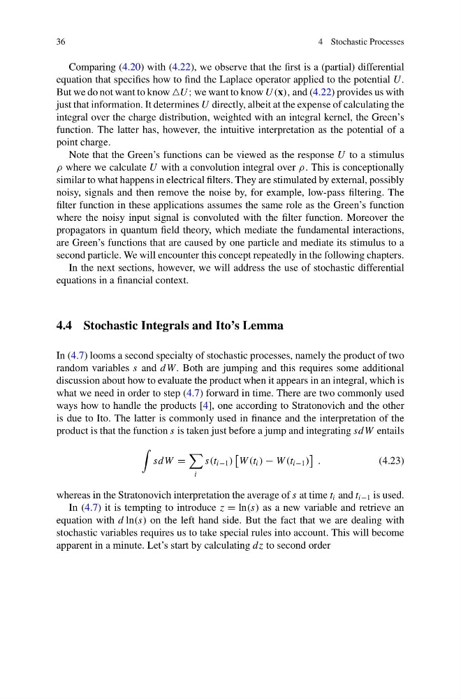
product is that the function s is taken just before a jump and integrating sdW entails
sdW =
i
s(t i−1 )
W (t i ) − W (t i−1 )
.
(4.23)
whereas in the Stratonovich interpretation the average of s at time t i and t i−1 is used.
In (4.7) it is tempting to introduce z = ln(s) as a new variable and retrieve an
equation with d ln(s) on the left hand side. But the fact that we are dealing with
stochastic variables requires us to take special rules into account. This will become
apparent in a minute. Let’s start by calculating dz to second order
4 Stochastic Processes
Comparing (4.20) with (4.22), we observe that the first is a (partial) differential
equation that specifies how to find the Laplace operator applied to the potential U.
But we do not want to know U ; we want to know U (x), and (4.22) provides us with
just that information. It determines U directly, albeit at the expense of calculating the
integral over the charge distribution, weighted with an integral kernel, the Green’s
function. The latter has, however, the intuitive interpretation as the potential of a
point charge.
Note that the Green’s functions can be viewed as the response U to a stimulus
ρ where we calculate U with a convolution integral over ρ. This is conceptionally
similar to what happens in electrical filters. They are stimulated by external, possibly
noisy, signals and then remove the noise by, for example, low-pass filtering. The
filter function in these applications assumes the same role as the Green’s function
where the noisy input signal is convoluted with the filter function. Moreover the
propagators in quantum field theory, which mediate the fundamental interactions,
are Green’s functions that are caused by one particle and mediate its stimulus to a
second particle. We will encounter this concept repeatedly in the following chapters.
In the next sections, however, we will address the use of stochastic differential
equations in a financial context.
4.4 Stochastic Integrals and Ito’s Lemma
In (4.7) looms a second specialty of stochastic processes, namely the product of two
random variables s and dW. Both are jumping and this requires some additional
discussion about how to evaluate the product when it appears in an integral, which is
what we need in order to step (4.7) forward in time. There are two commonly used
ways how to handle the products [4], one according to Stratonovich and the other
is due to Ito. The latter is commonly used in finance and the interpretation of the
product is that the function s is taken just before a jump and integrating sdW entails
sdW =
i
s(t i−1 )
W (t i ) − W (t i−1 )
.
(4.23)
whereas in the Stratonovich interpretation the average of s at time t i and t i−1 is used.
In (4.7) it is tempting to introduce z = ln(s) as a new variable and retrieve an
equation with d ln(s) on the left hand side. But the fact that we are dealing with
stochastic variables requires us to take special rules into account. This will become
apparent in a minute. Let’s start by calculating dz to second order