

3.2 Portfolio with Risky Assets Only
21
The point (σ
∗
, ρ
∗
) is indicated in Fig. 3.2 by an asterisk in the knee of the blue
curve. Note that the minimum is actually smaller than the smallest volatility of the
underlying assets, which was 1%. We find that mixing different shares can reduce the
volatility of the combined portfolio, though not eliminate it completely. Note also
that in some cases some of the weights w k can become negative, which corresponds
to shorting the asset with the negative weight.
In the derivation of the optimum portfolio distribution of shares w, we assumed
that the covariance matrix C is invertible, which is not the case if we include risk-free
assets such as government bonds in our portfolio. In the following section we relax
this constraint.
3.3 Portfolio with a Risk-Free Asset
If we have a risk-free asset available in our portfolio, the discussion in the previous
section up to (3.11) is unaffected, but inverting the covariance matrix C, which led
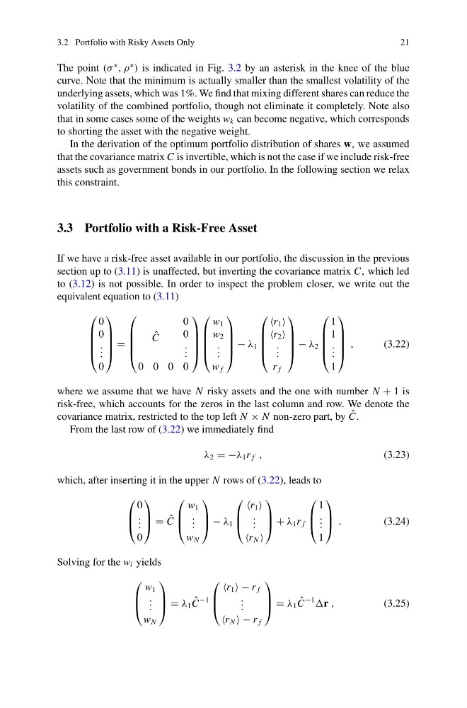
to (3.12) is not possible. In order to inspect the problem closer, we write out the
equivalent equation to (3.11)
⎛
⎜
⎜
⎜
⎝
0
0
. . .
0
⎞
⎟
⎟
⎟
⎠
=
⎛
⎜
⎜
⎜
⎝
ˆ
C
0
0
. . .
0 0 0 0
⎞
⎟
⎟
⎟
⎠
⎛
⎜
⎜
⎜
⎝
w 1
w 2
. . .
w f
⎞
⎟
⎟
⎟
⎠
− λ 1
⎛
⎜
⎜
⎜
⎝
r 1
r 2
. . .
r f
⎞
⎟
⎟
⎟
⎠
− λ 2
⎛
⎜
⎜
⎜
⎝
1
1
. . .
1
⎞
⎟
⎟
⎟
⎠
,
(3.22)
where we assume that we have N risky assets and the one with number N + 1 is
risk-free, which accounts for the zeros in the last column and row. We denote the
covariance matrix, restricted to the top left N × N non-zero part, by ˆ
C.
From the last row of (3.22) we immediately find
λ 2 = −λ 1 r f ,
(3.23)
which, after inserting it in the upper N rows of (3.22), leads to
⎛
⎜
⎝
0
. . .
0
⎞
⎟
⎠ = ˆ
C
⎛
⎜
⎝
w 1
. . .
w N
⎞
⎟
⎠ − λ 1
⎛
⎜
⎝
r 1
. . .
r N
⎞
⎟
⎠ + λ 1 r f
⎛
⎜
⎝
1
. . .
1
⎞
⎟
⎠ .
(3.24)
Solving for the w i yields
⎛
⎜
⎝
w 1
. . .
w N
⎞
⎟
⎠ = λ 1 ˆ
C
−1
⎛
⎜
⎝
r 1 − r f
. . .
r N − r f
⎞
⎟
⎠ = λ 1 ˆ
C
−1
r ,
(3.25)
21
The point (σ
∗
, ρ
∗
) is indicated in Fig. 3.2 by an asterisk in the knee of the blue
curve. Note that the minimum is actually smaller than the smallest volatility of the
underlying assets, which was 1%. We find that mixing different shares can reduce the
volatility of the combined portfolio, though not eliminate it completely. Note also
that in some cases some of the weights w k can become negative, which corresponds
to shorting the asset with the negative weight.
In the derivation of the optimum portfolio distribution of shares w, we assumed
that the covariance matrix C is invertible, which is not the case if we include risk-free
assets such as government bonds in our portfolio. In the following section we relax
this constraint.
3.3 Portfolio with a Risk-Free Asset
If we have a risk-free asset available in our portfolio, the discussion in the previous
section up to (3.11) is unaffected, but inverting the covariance matrix C, which led
to (3.12) is not possible. In order to inspect the problem closer, we write out the
equivalent equation to (3.11)
⎛
⎜
⎜
⎜
⎝
0
0
. . .
0
⎞
⎟
⎟
⎟
⎠
=
⎛
⎜
⎜
⎜
⎝
ˆ
C
0
0
. . .
0 0 0 0
⎞
⎟
⎟
⎟
⎠
⎛
⎜
⎜
⎜
⎝
w 1
w 2
. . .
w f
⎞
⎟
⎟
⎟
⎠
− λ 1
⎛
⎜
⎜
⎜
⎝
r 1
r 2
. . .
r f
⎞
⎟
⎟
⎟
⎠
− λ 2
⎛
⎜
⎜
⎜
⎝
1
1
. . .
1
⎞
⎟
⎟
⎟
⎠
,
(3.22)
where we assume that we have N risky assets and the one with number N + 1 is
risk-free, which accounts for the zeros in the last column and row. We denote the
covariance matrix, restricted to the top left N × N non-zero part, by ˆ
C.
From the last row of (3.22) we immediately find
λ 2 = −λ 1 r f ,
(3.23)
which, after inserting it in the upper N rows of (3.22), leads to
⎛
⎜
⎝
0
. . .
0
⎞
⎟
⎠ = ˆ
C
⎛
⎜
⎝
w 1
. . .
w N
⎞
⎟
⎠ − λ 1
⎛
⎜
⎝
r 1
. . .
r N
⎞
⎟
⎠ + λ 1 r f
⎛
⎜
⎝
1
. . .
1
⎞
⎟
⎠ .
(3.24)
Solving for the w i yields
⎛
⎜
⎝
w 1
. . .
w N
⎞
⎟
⎠ = λ 1 ˆ
C
−1
⎛
⎜
⎝
r 1 − r f
. . .
r N − r f
⎞
⎟
⎠ = λ 1 ˆ
C
−1
r ,
(3.25)