

22
3 Portfolio Theory and CAPM
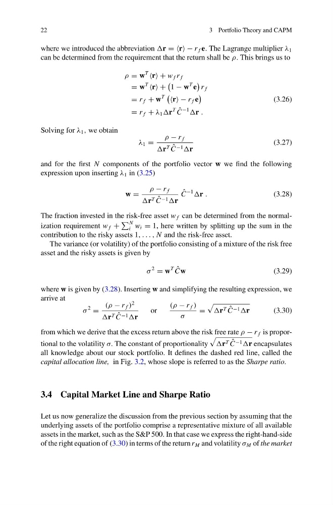
where we introduced the abbreviation r = =r − r f e. The Lagrange multiplier λ 1
can be determined from the requirement that the return shall be ρ. This brings us to
ρ = w
T
r + w f r f
= w
T
r +
1 − w
T e
r f
= r f + w
T
r − r f e
(3.26)
= r f + λ 1 r
T ˆ
C
−1
r .
Solving for λ 1 , we obtain
λ 1 =
ρ − r f
r T ˆ
C −1 r
(3.27)
and for the first N components of the portfolio vector w we find the following
expression upon inserting λ 1 in (3.25)
w =
ρ − r f
r T ˆ
C −1 r
ˆ
C
−1
r .
(3.28)
The fraction invested in the risk-free asset w f can be determined from the normalization requirement w f +
N
i w i = 1, here written by splitting up the sum in the
contribution to the risky assets 1, . . . , N and the risk-free asset.
The variance (or volatility) of the portfolio consisting of a mixture of the risk free
asset and the risky assets is given by
σ
2
= w
T ˆ
Cw
(3.29)
where w is given by (3.28). Inserting w and simplifying the resulting expression, we
arrive at
σ
2
=
(ρ − r f )
2
r T ˆ
C −1 r
or
(ρ − r f )
σ
=
r T ˆ
C −1 r
(3.30)
from which we derive that the excess return above the risk free rate ρ − r f is proportional to the volatility σ. The constant of proportionality
r T ˆ
C −1 r encapsulates
all knowledge about our stock portfolio. It defines the dashed red line, called the
capital allocation line, in Fig. 3.2, whose slope is referred to as the Sharpe ratio.
3.4 Capital Market Line and Sharpe Ratio
Let us now generalize the discussion from the previous section by assuming that the
underlying assets of the portfolio comprise a representative mixture of all available
assets in the market, such as the S&P 500. In that case we express the right-hand-side
of the right equation of (3.30) in terms of the return r M and volatility σ M of the market
3 Portfolio Theory and CAPM
where we introduced the abbreviation r = =r − r f e. The Lagrange multiplier λ 1
can be determined from the requirement that the return shall be ρ. This brings us to
ρ = w
T
r + w f r f
= w
T
r +
1 − w
T e
r f
= r f + w
T
r − r f e
(3.26)
= r f + λ 1 r
T ˆ
C
−1
r .
Solving for λ 1 , we obtain
λ 1 =
ρ − r f
r T ˆ
C −1 r
(3.27)
and for the first N components of the portfolio vector w we find the following
expression upon inserting λ 1 in (3.25)
w =
ρ − r f
r T ˆ
C −1 r
ˆ
C
−1
r .
(3.28)
The fraction invested in the risk-free asset w f can be determined from the normalization requirement w f +
N
i w i = 1, here written by splitting up the sum in the
contribution to the risky assets 1, . . . , N and the risk-free asset.
The variance (or volatility) of the portfolio consisting of a mixture of the risk free
asset and the risky assets is given by
σ
2
= w
T ˆ
Cw
(3.29)
where w is given by (3.28). Inserting w and simplifying the resulting expression, we
arrive at
σ
2
=
(ρ − r f )
2
r T ˆ
C −1 r
or
(ρ − r f )
σ
=
r T ˆ
C −1 r
(3.30)
from which we derive that the excess return above the risk free rate ρ − r f is proportional to the volatility σ. The constant of proportionality
r T ˆ
C −1 r encapsulates
all knowledge about our stock portfolio. It defines the dashed red line, called the
capital allocation line, in Fig. 3.2, whose slope is referred to as the Sharpe ratio.
3.4 Capital Market Line and Sharpe Ratio
Let us now generalize the discussion from the previous section by assuming that the
underlying assets of the portfolio comprise a representative mixture of all available
assets in the market, such as the S&P 500. In that case we express the right-hand-side
of the right equation of (3.30) in terms of the return r M and volatility σ M of the market