

20
3 Portfolio Theory and CAPM
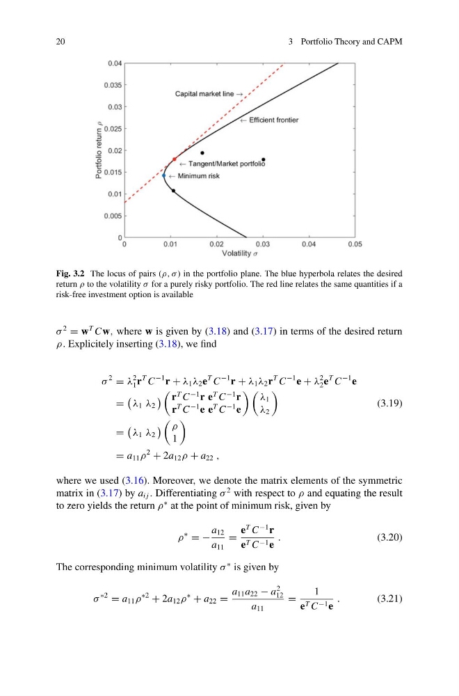
Fig. 3.2 The locus of pairs (ρ, σ ) in the portfolio plane. The blue hyperbola relates the desired
return ρ to the volatility σ for a purely risky portfolio. The red line relates the same quantities if a
risk-free investment option is available
σ
2
= w
T Cw, where w is given by (3.18) and (3.17) in terms of the desired return
ρ. Explicitely inserting (3.18), we find
σ
2
= λ
2
1 r
T C
−1 r + λ 1 λ 2 e
T C
−1 r + λ 1 λ 2 r
T C
−1 e + λ
2
2 e
T C
−1 e
=
λ 1 λ 2
r
T C
−1 r e
T C
−1 r
r
T C
−1 e e
T C
−1 e
λ 1
λ 2
(3.19)
=
λ 1 λ 2
ρ
1
= a 11 ρ
2
+ 2a 12 ρ + a 22 ,
where we used (3.16). Moreover, we denote the matrix elements of the symmetric
matrix in (3.17) by a i j . Differentiating σ
2 with respect to ρ and equating the result
to zero yields the return ρ
∗ at the point of minimum risk, given by
ρ
∗
= −
a 12
a 11
=
e
T C
−1 r
e T C −1 e
.
(3.20)
The corresponding minimum volatility σ
∗ is given by
σ
∗2
= a 11 ρ
∗2
+ 2a 12 ρ
∗
+ a 22 =
a 11 a 22 − a
2
12
a 11
=
1
e T C −1 e
.
(3.21)
3 Portfolio Theory and CAPM
Fig. 3.2 The locus of pairs (ρ, σ ) in the portfolio plane. The blue hyperbola relates the desired
return ρ to the volatility σ for a purely risky portfolio. The red line relates the same quantities if a
risk-free investment option is available
σ
2
= w
T Cw, where w is given by (3.18) and (3.17) in terms of the desired return
ρ. Explicitely inserting (3.18), we find
σ
2
= λ
2
1 r
T C
−1 r + λ 1 λ 2 e
T C
−1 r + λ 1 λ 2 r
T C
−1 e + λ
2
2 e
T C
−1 e
=
λ 1 λ 2
r
T C
−1 r e
T C
−1 r
r
T C
−1 e e
T C
−1 e
λ 1
λ 2
(3.19)
=
λ 1 λ 2
ρ
1
= a 11 ρ
2
+ 2a 12 ρ + a 22 ,
where we used (3.16). Moreover, we denote the matrix elements of the symmetric
matrix in (3.17) by a i j . Differentiating σ
2 with respect to ρ and equating the result
to zero yields the return ρ
∗ at the point of minimum risk, given by
ρ
∗
= −
a 12
a 11
=
e
T C
−1 r
e T C −1 e
.
(3.20)
The corresponding minimum volatility σ
∗ is given by
σ
∗2
= a 11 ρ
∗2
+ 2a 12 ρ
∗
+ a 22 =
a 11 a 22 − a
2
12
a 11
=
1
e T C −1 e
.
(3.21)