

162
10 Quantum Finance and Path Integrals
S BS = ε
N
i=1
L BS (i) = ε
N
i=1
L BS (x i , x i−1 , ε)
(10.62)
= −
1
2σ 2 ε
N
i=1
x i − x i−1 + ε
r f −
σ
2
2
2
− εr f N .
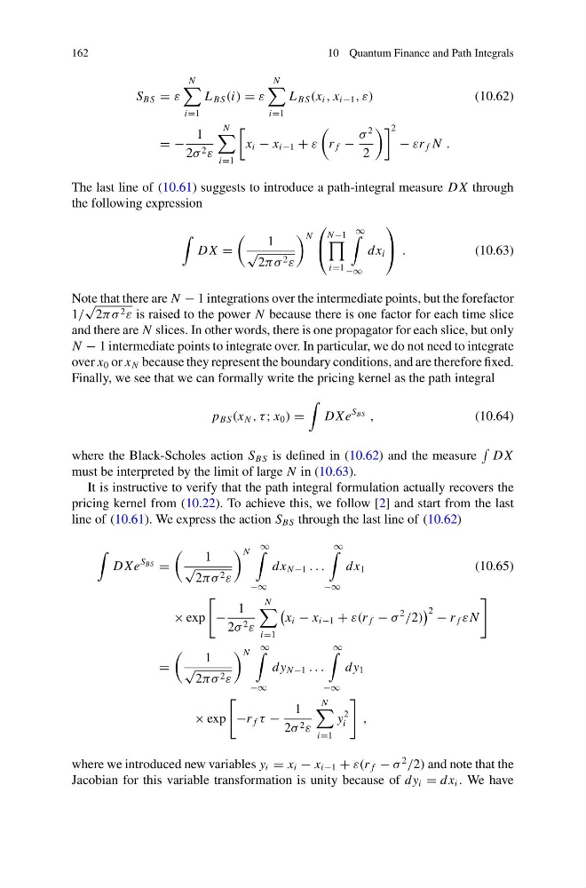
The last line of (10.61) suggests to introduce a path-integral measure D X through
the following expression
D X =
1
√
2πσ 2 ε
N
⎛
⎝
N −1
i=1
∞
−∞
dx i
⎞
⎠ .
(10.63)
Note that there are N − 1 integrations over the intermediate points, but the forefactor
1/
√
2πσ 2 ε is raised to the power N because there is one factor for each time slice
and there are N slices. In other words, there is one propagator for each slice, but only
N − 1 intermediate points to integrate over. In particular, we do not need to integrate
over x 0 or x N because they represent the boundary conditions, and are therefore fixed.
Finally, we see that we can formally write the pricing kernel as the path integral
p BS (x N , τ ; x 0 ) =
D Xe
S BS ,
(10.64)
where the Black-Scholes action S BS is defined in (10.62) and the measure
D X
must be interpreted by the limit of large N in (10.63).
It is instructive to verify that the path integral formulation actually recovers the
pricing kernel from (10.22). To achieve this, we follow [2] and start from the last
line of (10.61). We express the action S BS through the last line of (10.62)
D Xe
S BS =
1
√
2πσ 2 ε
N
∞
−∞
dx N −1 . . .
∞
−∞
dx 1
(10.65)
× exp
−
1
2σ 2 ε
N
i=1
x i − x i−1 + ε(r f − σ
2
/2)
2 − r f εN
=
1
√
2πσ 2 ε
N
∞
−∞
dy N −1 . . .
∞
−∞
dy 1
× exp
−r f τ −
1
2σ 2 ε
N
i=1
y
2
i
,
where we introduced new variables y i = x i − x i−1 + ε(r f − σ
2
/2) and note that the
Jacobian for this variable transformation is unity because of dy i = dx i . We have
10 Quantum Finance and Path Integrals
S BS = ε
N
i=1
L BS (i) = ε
N
i=1
L BS (x i , x i−1 , ε)
(10.62)
= −
1
2σ 2 ε
N
i=1
x i − x i−1 + ε
r f −
σ
2
2
2
− εr f N .
The last line of (10.61) suggests to introduce a path-integral measure D X through
the following expression
D X =
1
√
2πσ 2 ε
N
⎛
⎝
N −1
i=1
∞
−∞
dx i
⎞
⎠ .
(10.63)
Note that there are N − 1 integrations over the intermediate points, but the forefactor
1/
√
2πσ 2 ε is raised to the power N because there is one factor for each time slice
and there are N slices. In other words, there is one propagator for each slice, but only
N − 1 intermediate points to integrate over. In particular, we do not need to integrate
over x 0 or x N because they represent the boundary conditions, and are therefore fixed.
Finally, we see that we can formally write the pricing kernel as the path integral
p BS (x N , τ ; x 0 ) =
D Xe
S BS ,
(10.64)
where the Black-Scholes action S BS is defined in (10.62) and the measure
D X
must be interpreted by the limit of large N in (10.63).
It is instructive to verify that the path integral formulation actually recovers the
pricing kernel from (10.22). To achieve this, we follow [2] and start from the last
line of (10.61). We express the action S BS through the last line of (10.62)
D Xe
S BS =
1
√
2πσ 2 ε
N
∞
−∞
dx N −1 . . .
∞
−∞
dx 1
(10.65)
× exp
−
1
2σ 2 ε
N
i=1
x i − x i−1 + ε(r f − σ
2
/2)
2 − r f εN
=
1
√
2πσ 2 ε
N
∞
−∞
dy N −1 . . .
∞
−∞
dy 1
× exp
−r f τ −
1
2σ 2 ε
N
i=1
y
2
i
,
where we introduced new variables y i = x i − x i−1 + ε(r f − σ
2
/2) and note that the
Jacobian for this variable transformation is unity because of dy i = dx i . We have