

10.6 Path Integrals in Finance
161
The other equation of motion yields ∂ H BS /∂ x = 0 because the Black-Scholes Hamiltonian H BS does not explicitely depend on x.
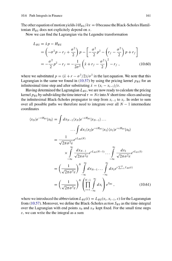
Now we can find the Lagrangian via the Legendre transformation
L BS = ˙
x p − H BS
=
−σ
2 p − r f +
σ
2
2
p −
−
σ
2
2
p
2
−
r f −
σ
2
2
p + r f
= −
σ
2
2
p
2
− r f = −
1
2σ 2
˙
x + r f −
σ
2
2
2
− r f ,
(10.60)
where we substituted p = ( ˙
x + r − σ
2
/2)/σ
2 in the last equation. We note that this
Lagrangian is the same we found in (10.57) by using the pricing kernel p BS for an
infinitesimal time step and after substituting ˙
x = (x i − x i−1 )/ε.
Having determined the Lagrangian L BS , we are now ready to calculate the pricing
kernel p BS by subdividing the time interval τ = N ε into N short time-slices and using
the infinitesimal Black-Scholes propagator to step from x i−1 to x i . In order to sum
over all possible paths we therefore need to integrate over all N − 1 intermediate
coordinates
x N |e
−τ H BS |x 0 =
dx N −1 x N |e
−ε H BS |x N −1 . . .
. . .
dx 1 x 2 |e
−ε H BS |x 1 x 1 |e
−ε H BS |x 0
=
1
√
2πσ 2 ε
e
εL BS (N )
×
∞
−∞
dx N −1
√
2πσ 2 ε
e
εL BS (N −1)
. . .
∞
−∞
dx 1
√
2πσ 2 ε
e
εL BS (1)
=
1
√
2πσ 2 ε
N
∞
−∞
dx N −1 . . .
∞
−∞
dx 1 e
ε
N
i=1 L BS (i)
=
1
√
2πσ 2 ε
N
⎛
⎝
N −1
i=1
∞
−∞
dx i
⎞
⎠ e
S BS ,
(10.61)
where we introduced the abbreviation L BS (i) = L BS (x i , x i−1 , ε) for the Lagarangian
from (10.57). Moreover, we define the Black-Scholes action S BS as the time-integral
over the Lagrangian with end points x 0 and x N kept fixed. For the small time steps
ε, we can write the the integral as a sum
161
The other equation of motion yields ∂ H BS /∂ x = 0 because the Black-Scholes Hamiltonian H BS does not explicitely depend on x.
Now we can find the Lagrangian via the Legendre transformation
L BS = ˙
x p − H BS
=
−σ
2 p − r f +
σ
2
2
p −
−
σ
2
2
p
2
−
r f −
σ
2
2
p + r f
= −
σ
2
2
p
2
− r f = −
1
2σ 2
˙
x + r f −
σ
2
2
2
− r f ,
(10.60)
where we substituted p = ( ˙
x + r − σ
2
/2)/σ
2 in the last equation. We note that this
Lagrangian is the same we found in (10.57) by using the pricing kernel p BS for an
infinitesimal time step and after substituting ˙
x = (x i − x i−1 )/ε.
Having determined the Lagrangian L BS , we are now ready to calculate the pricing
kernel p BS by subdividing the time interval τ = N ε into N short time-slices and using
the infinitesimal Black-Scholes propagator to step from x i−1 to x i . In order to sum
over all possible paths we therefore need to integrate over all N − 1 intermediate
coordinates
x N |e
−τ H BS |x 0 =
dx N −1 x N |e
−ε H BS |x N −1 . . .
. . .
dx 1 x 2 |e
−ε H BS |x 1 x 1 |e
−ε H BS |x 0
=
1
√
2πσ 2 ε
e
εL BS (N )
×
∞
−∞
dx N −1
√
2πσ 2 ε
e
εL BS (N −1)
. . .
∞
−∞
dx 1
√
2πσ 2 ε
e
εL BS (1)
=
1
√
2πσ 2 ε
N
∞
−∞
dx N −1 . . .
∞
−∞
dx 1 e
ε
N
i=1 L BS (i)
=
1
√
2πσ 2 ε
N
⎛
⎝
N −1
i=1
∞
−∞
dx i
⎞
⎠ e
S BS ,
(10.61)
where we introduced the abbreviation L BS (i) = L BS (x i , x i−1 , ε) for the Lagarangian
from (10.57). Moreover, we define the Black-Scholes action S BS as the time-integral
over the Lagrangian with end points x 0 and x N kept fixed. For the small time steps
ε, we can write the the integral as a sum