

160
10 Quantum Finance and Path Integrals
Lagrangian to the Hamiltonian in the Schrödinger equation. Note also that the calculations we performed in the last part of this section resembled the steps to derived
the Fokker-Planck equation from the Master equation in Sect. 4.5. This observation
should justify the daring step to apply path integrals to finance.
10.6 Path Integrals in Finance
In this section we will re-derive the pricing kernel p BS from (10.22) for the BlackScholes Hamiltonian with the help of path integrals, first used in the context of
finance by Dash [5], to illustrate the methodology. In the previous section, we found
that the path integral depends on the action in the exponent, where the action is the
integral over the Lagrangian from fixed starting and end points at fixed initial and
final times. So how do we find the Lagrangian that corresponds to the Black-Scholes
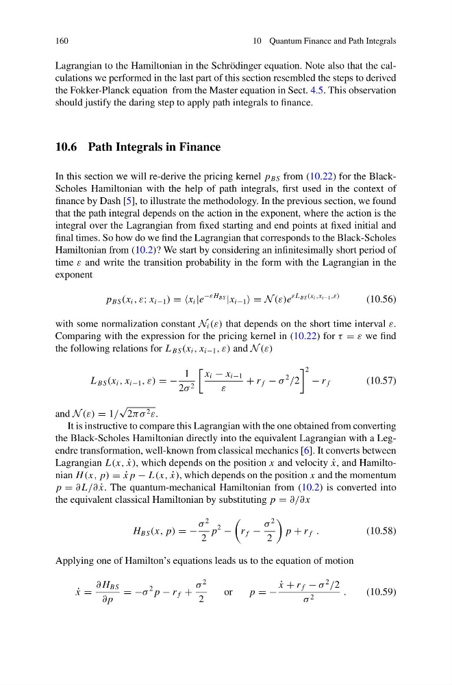
Hamiltonian from (10.2)? We start by considering an infinitesimally short period of
time ε and write the transition probability in the form with the Lagrangian in the
exponent
p BS (x i , ε; x i−1 ) = =x i |e
−ε H BS |x i−1 = N (ε)e
εL BS (x i ,x i−1 ,ε)
(10.56)
with some normalization constant N i (ε) that depends on the short time interval ε.
Comparing with the expression for the pricing kernel in (10.22) for τ = ε we find
the following relations for L BS (x i , x i−1 , ε) and N (ε)
L BS (x i , x i−1 , ε) = −
1
2σ 2
x i − x i−1
ε
+ r f − σ
2
/2
2
− r f
(10.57)
and N (ε) = 1/
√
2πσ 2 ε.
It is instructive to compare this Lagrangian with the one obtained from converting
the Black-Scholes Hamiltonian directly into the equivalent Lagrangian with a Legendre transformation, well-known from classical mechanics [6]. It converts between
Lagrangian L(x, ˙
x), which depends on the position x and velocity ˙
x, and Hamiltonian H (x, p) = ˙
x p − L(x, ˙
x), which depends on the position x and the momentum
p = ∂ L/∂ ˙
x. The quantum-mechanical Hamiltonian from (10.2) is converted into
the equivalent classical Hamiltonian by substituting p = ∂/∂ x
H BS (x, p) = −
σ
2
2
p
2
−
r f −
σ
2
2
p + r f .
(10.58)
Applying one of Hamilton’s equations leads us to the equation of motion
˙
x =
∂ H BS
∂ p
= −σ
2 p − r f +
σ
2
2
or
p = −
˙
x + r f − σ
2
/2
σ 2
.
(10.59)
10 Quantum Finance and Path Integrals
Lagrangian to the Hamiltonian in the Schrödinger equation. Note also that the calculations we performed in the last part of this section resembled the steps to derived
the Fokker-Planck equation from the Master equation in Sect. 4.5. This observation
should justify the daring step to apply path integrals to finance.
10.6 Path Integrals in Finance
In this section we will re-derive the pricing kernel p BS from (10.22) for the BlackScholes Hamiltonian with the help of path integrals, first used in the context of
finance by Dash [5], to illustrate the methodology. In the previous section, we found
that the path integral depends on the action in the exponent, where the action is the
integral over the Lagrangian from fixed starting and end points at fixed initial and
final times. So how do we find the Lagrangian that corresponds to the Black-Scholes
Hamiltonian from (10.2)? We start by considering an infinitesimally short period of
time ε and write the transition probability in the form with the Lagrangian in the
exponent
p BS (x i , ε; x i−1 ) = =x i |e
−ε H BS |x i−1 = N (ε)e
εL BS (x i ,x i−1 ,ε)
(10.56)
with some normalization constant N i (ε) that depends on the short time interval ε.
Comparing with the expression for the pricing kernel in (10.22) for τ = ε we find
the following relations for L BS (x i , x i−1 , ε) and N (ε)
L BS (x i , x i−1 , ε) = −
1
2σ 2
x i − x i−1
ε
+ r f − σ
2
/2
2
− r f
(10.57)
and N (ε) = 1/
√
2πσ 2 ε.
It is instructive to compare this Lagrangian with the one obtained from converting
the Black-Scholes Hamiltonian directly into the equivalent Lagrangian with a Legendre transformation, well-known from classical mechanics [6]. It converts between
Lagrangian L(x, ˙
x), which depends on the position x and velocity ˙
x, and Hamiltonian H (x, p) = ˙
x p − L(x, ˙
x), which depends on the position x and the momentum
p = ∂ L/∂ ˙
x. The quantum-mechanical Hamiltonian from (10.2) is converted into
the equivalent classical Hamiltonian by substituting p = ∂/∂ x
H BS (x, p) = −
σ
2
2
p
2
−
r f −
σ
2
2
p + r f .
(10.58)
Applying one of Hamilton’s equations leads us to the equation of motion
˙
x =
∂ H BS
∂ p
= −σ
2 p − r f +
σ
2
2
or
p = −
˙
x + r f − σ
2
/2
σ 2
.
(10.59)