

10.5 Path Integrals in Quantum Mechanics
159
ψ(x, t) + ε
∂ψ
∂t
=
1
A
∞
−∞
exp
imξ 2
ε
1 −
iεV (x)
ψ(x + ξ, t)dξ
(10.51)
=
1
A
∞
−∞
exp
imξ 2
ε
1 −
iεV (x)
ψ(x, t) + ξ
∂ψ
∂ x
+
ξ 2
2
∂ 2 ψ
∂ x 2
dξ ,
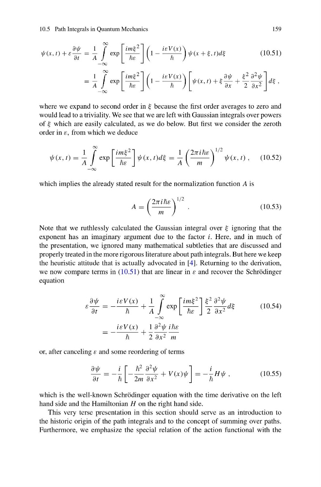
where we expand to second order in ξ because the first order averages to zero and
would lead to a triviality. We see that we are left with Gaussian integrals over powers
of ξ which are easily calculated, as we do below. But first we consider the zeroth
order in ε, from which we deduce
ψ(x, t) =
1
A
∞
−∞
exp
imξ
2
ε
ψ(x, t)dξ =
1
A
2πiε
m
1/2
ψ(x, t) , (10.52)
which implies the already stated result for the normalization function A is
A =
2πiε
m
1/2
.
(10.53)
Note that we ruthlessly calculated the Gaussian integral over ξ ignoring that the
exponent has an imaginary argument due to the factor i. Here, and in much of
the presentation, we ignored many mathematical subtleties that are discussed and
properly treated in the more rigorous literature about path integrals. But here we keep
the heuristic attitude that is actually advocated in [4]. Returning to the derivation,
we now compare terms in (10.51) that are linear in ε and recover the Schrödinger
equation
ε
∂ψ
∂t
= −
iεV (x)
+
1
A
∞
−∞
exp
imξ
2
ε
ξ
2
2
∂
2
ψ
∂ x 2 dξ
(10.54)
= −
iεV (x)
+
1
2
∂
2
ψ
∂ x 2
iε
m
or, after canceling ε and some reordering of terms
∂ψ
∂t
= −
i
−
2
2m
∂
2
ψ
∂ x 2 + V (x)ψ
= −
i
H ψ ,
(10.55)
which is the well-known Schrödinger equation with the time derivative on the left
hand side and the Hamiltonian H on the right hand side.
This very terse presentation in this section should serve as an introduction to
the historic origin of the path integrals and to the concept of summing over paths.
Furthermore, we emphasize the special relation of the action functional with the
159
ψ(x, t) + ε
∂ψ
∂t
=
1
A
∞
−∞
exp
imξ 2
ε
1 −
iεV (x)
ψ(x + ξ, t)dξ
(10.51)
=
1
A
∞
−∞
exp
imξ 2
ε
1 −
iεV (x)
ψ(x, t) + ξ
∂ψ
∂ x
+
ξ 2
2
∂ 2 ψ
∂ x 2
dξ ,
where we expand to second order in ξ because the first order averages to zero and
would lead to a triviality. We see that we are left with Gaussian integrals over powers
of ξ which are easily calculated, as we do below. But first we consider the zeroth
order in ε, from which we deduce
ψ(x, t) =
1
A
∞
−∞
exp
imξ
2
ε
ψ(x, t)dξ =
1
A
2πiε
m
1/2
ψ(x, t) , (10.52)
which implies the already stated result for the normalization function A is
A =
2πiε
m
1/2
.
(10.53)
Note that we ruthlessly calculated the Gaussian integral over ξ ignoring that the
exponent has an imaginary argument due to the factor i. Here, and in much of
the presentation, we ignored many mathematical subtleties that are discussed and
properly treated in the more rigorous literature about path integrals. But here we keep
the heuristic attitude that is actually advocated in [4]. Returning to the derivation,
we now compare terms in (10.51) that are linear in ε and recover the Schrödinger
equation
ε
∂ψ
∂t
= −
iεV (x)
+
1
A
∞
−∞
exp
imξ
2
ε
ξ
2
2
∂
2
ψ
∂ x 2 dξ
(10.54)
= −
iεV (x)
+
1
2
∂
2
ψ
∂ x 2
iε
m
or, after canceling ε and some reordering of terms
∂ψ
∂t
= −
i
−
2
2m
∂
2
ψ
∂ x 2 + V (x)ψ
= −
i
H ψ ,
(10.55)
which is the well-known Schrödinger equation with the time derivative on the left
hand side and the Hamiltonian H on the right hand side.
This very terse presentation in this section should serve as an introduction to
the historic origin of the path integrals and to the concept of summing over paths.
Furthermore, we emphasize the special relation of the action functional with the