

140
9 Bubbles, Crashes, Fat Tails and Lévy-Stable Distributions
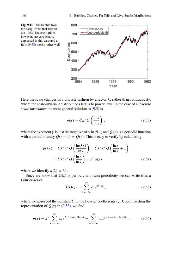
Fig. 9.15 The bubble from
the early 1960s that fizzled
out 1962. The oscillations,
however, are very clearly
expressed in this case and a
fit to (9.58) works rather well
Here the scale changes in a discrete fashion by a factor λ, rather than continuously,
where the scale-invariant distributions led us to power laws. In the case of a discrete
scale invariance the most general solution to (9.5) is
p(x) = ˆ
C x
γ Q
ln x
ln λ
,
(9.53)
where the exponent γ is just the negative of α in (9.1) and Q(x) is a periodic function
with a period of unity Q(z + 1) = Q(z). This is easy to verify by calculating
p(λx) = ˆ
Cλ
γ x
γ Q
ln(λx)
ln λ
= ˆ
Cλ
γ x
γ Q
ln x
ln λ
+ 1
= ˆ
Cλ
γ x
γ Q
ln x
ln λ
= λ
γ p(x)
(9.54)
where we identify q(λ) = λ
γ
.
Since we know that Q(z) is periodic with unit periodicity we can write it as a
Fourier-series
ˆ
C Q(z) =
∞
n=−∞
c n e
2πinz
,
(9.55)
where we absorbed the constant ˆ
C in the Fourier coefficients c n . Upon inserting the
representation of Q(z) in (9.53), we find
p(x) = x
γ
∞
n=−∞
c n e
2πin ln(x)/ ln(λ)
=
∞
n=−∞
c n x
γ +2πin ln(x)/ ln(λ)
,
(9.56)
9 Bubbles, Crashes, Fat Tails and Lévy-Stable Distributions
Fig. 9.15 The bubble from
the early 1960s that fizzled
out 1962. The oscillations,
however, are very clearly
expressed in this case and a
fit to (9.58) works rather well
Here the scale changes in a discrete fashion by a factor λ, rather than continuously,
where the scale-invariant distributions led us to power laws. In the case of a discrete
scale invariance the most general solution to (9.5) is
p(x) = ˆ
C x
γ Q
ln x
ln λ
,
(9.53)
where the exponent γ is just the negative of α in (9.1) and Q(x) is a periodic function
with a period of unity Q(z + 1) = Q(z). This is easy to verify by calculating
p(λx) = ˆ
Cλ
γ x
γ Q
ln(λx)
ln λ
= ˆ
Cλ
γ x
γ Q
ln x
ln λ
+ 1
= ˆ
Cλ
γ x
γ Q
ln x
ln λ
= λ
γ p(x)
(9.54)
where we identify q(λ) = λ
γ
.
Since we know that Q(z) is periodic with unit periodicity we can write it as a
Fourier-series
ˆ
C Q(z) =
∞
n=−∞
c n e
2πinz
,
(9.55)
where we absorbed the constant ˆ
C in the Fourier coefficients c n . Upon inserting the
representation of Q(z) in (9.53), we find
p(x) = x
γ
∞
n=−∞
c n e
2πin ln(x)/ ln(λ)
=
∞
n=−∞
c n x
γ +2πin ln(x)/ ln(λ)
,
(9.56)