

9.10 Finite-Time Divergence and Log-Periodic Oscillations
139
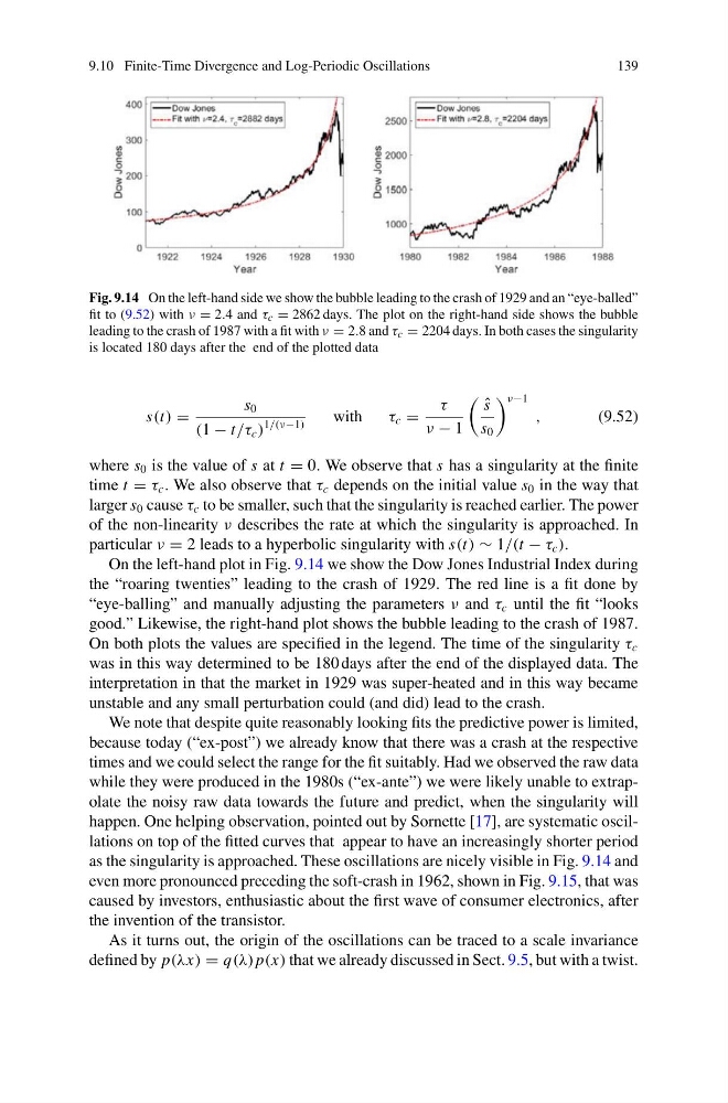
Fig. 9.14 On the left-hand side we show the bubble leading to the crash of 1929 and an “eye-balled”
fit to (9.52) with ν = 2.4 and τ c = 2862 days. The plot on the right-hand side shows the bubble
leading to the crash of 1987 with a fit with ν = 2.8 and τ c = 2204 days. In both cases the singularity
is located 180 days after the end of the plotted data
s(t) =
s 0
(1 − t/τ c )
1/(ν−1)
with
τ c =
τ
ν − 1
ˆ
s
s 0
ν−1
,
(9.52)
where s 0 is the value of s at t = 0. We observe that s has a singularity at the finite
time t = τ c . We also observe that τ c depends on the initial value s 0 in the way that
larger s 0 cause τ c to be smaller, such that the singularity is reached earlier. The power
of the non-linearity ν describes the rate at which the singularity is approached. In
particular ν = 2 leads to a hyperbolic singularity with s(t) ∼ 1/(t − τ c ).
On the left-hand plot in Fig. 9.14 we show the Dow Jones Industrial Index during
the “roaring twenties” leading to the crash of 1929. The red line is a fit done by
“eye-balling” and manually adjusting the parameters ν and τ c until the fit “looks
good.” Likewise, the right-hand plot shows the bubble leading to the crash of 1987.
On both plots the values are specified in the legend. The time of the singularity τ c
was in this way determined to be 180 days after the end of the displayed data. The
interpretation in that the market in 1929 was super-heated and in this way became
unstable and any small perturbation could (and did) lead to the crash.
We note that despite quite reasonably looking fits the predictive power is limited,
because today (“ex-post”) we already know that there was a crash at the respective
times and we could select the range for the fit suitably. Had we observed the raw data
while they were produced in the 1980s (“ex-ante”) we were likely unable to extrapolate the noisy raw data towards the future and predict, when the singularity will
happen. One helping observation, pointed out by Sornette [17], are systematic oscillations on top of the fitted curves that appear to have an increasingly shorter period
as the singularity is approached. These oscillations are nicely visible in Fig. 9.14 and
even more pronounced preceding the soft-crash in 1962, shown in Fig. 9.15, that was
caused by investors, enthusiastic about the first wave of consumer electronics, after
the invention of the transistor.
As it turns out, the origin of the oscillations can be traced to a scale invariance
defined by p(λx) = q(λ) p(x) that we already discussed in Sect. 9.5, but with a twist.
139
Fig. 9.14 On the left-hand side we show the bubble leading to the crash of 1929 and an “eye-balled”
fit to (9.52) with ν = 2.4 and τ c = 2862 days. The plot on the right-hand side shows the bubble
leading to the crash of 1987 with a fit with ν = 2.8 and τ c = 2204 days. In both cases the singularity
is located 180 days after the end of the plotted data
s(t) =
s 0
(1 − t/τ c )
1/(ν−1)
with
τ c =
τ
ν − 1
ˆ
s
s 0
ν−1
,
(9.52)
where s 0 is the value of s at t = 0. We observe that s has a singularity at the finite
time t = τ c . We also observe that τ c depends on the initial value s 0 in the way that
larger s 0 cause τ c to be smaller, such that the singularity is reached earlier. The power
of the non-linearity ν describes the rate at which the singularity is approached. In
particular ν = 2 leads to a hyperbolic singularity with s(t) ∼ 1/(t − τ c ).
On the left-hand plot in Fig. 9.14 we show the Dow Jones Industrial Index during
the “roaring twenties” leading to the crash of 1929. The red line is a fit done by
“eye-balling” and manually adjusting the parameters ν and τ c until the fit “looks
good.” Likewise, the right-hand plot shows the bubble leading to the crash of 1987.
On both plots the values are specified in the legend. The time of the singularity τ c
was in this way determined to be 180 days after the end of the displayed data. The
interpretation in that the market in 1929 was super-heated and in this way became
unstable and any small perturbation could (and did) lead to the crash.
We note that despite quite reasonably looking fits the predictive power is limited,
because today (“ex-post”) we already know that there was a crash at the respective
times and we could select the range for the fit suitably. Had we observed the raw data
while they were produced in the 1980s (“ex-ante”) we were likely unable to extrapolate the noisy raw data towards the future and predict, when the singularity will
happen. One helping observation, pointed out by Sornette [17], are systematic oscillations on top of the fitted curves that appear to have an increasingly shorter period
as the singularity is approached. These oscillations are nicely visible in Fig. 9.14 and
even more pronounced preceding the soft-crash in 1962, shown in Fig. 9.15, that was
caused by investors, enthusiastic about the first wave of consumer electronics, after
the invention of the transistor.
As it turns out, the origin of the oscillations can be traced to a scale invariance
defined by p(λx) = q(λ) p(x) that we already discussed in Sect. 9.5, but with a twist.