

9.10 Finite-Time Divergence and Log-Periodic Oscillations
141
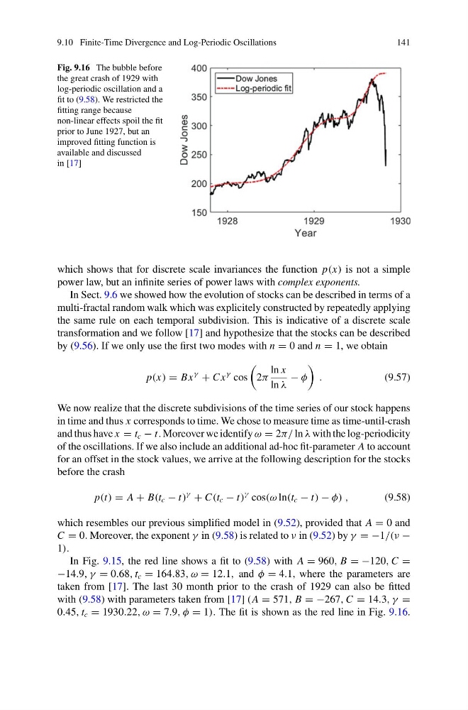
Fig. 9.16 The bubble before
the great crash of 1929 with
log-periodic oscillation and a
fit to (9.58). We restricted the
fitting range because
non-linear effects spoil the fit
prior to June 1927, but an
improved fitting function is
available and discussed
in [17]
which shows that for discrete scale invariances the function p(x) is not a simple
power law, but an infinite series of power laws with complex exponents.
In Sect. 9.6 we showed how the evolution of stocks can be described in terms of a
multi-fractal random walk which was explicitely constructed by repeatedly applying
the same rule on each temporal subdivision. This is indicative of a discrete scale
transformation and we follow [17] and hypothesize that the stocks can be described
by (9.56). If we only use the first two modes with n = 0 and n = 1, we obtain
p(x) = Bx
γ
+ C x
γ cos
2π
ln x
ln λ
− φ
.
(9.57)
We now realize that the discrete subdivisions of the time series of our stock happens
in time and thus x corresponds to time. We chose to measure time as time-until-crash
and thus have x = t c − t. Moreover we identify ω = 2π/ ln λ with the log-periodicity
of the oscillations. If we also include an additional ad-hoc fit-parameter A to account
for an offset in the stock values, we arrive at the following description for the stocks
before the crash
p(t) = A + B(t c − t)
γ
+ C(t c − t)
γ cos(ω ln(t c − t) − φ) ,
(9.58)
which resembles our previous simplified model in (9.52), provided that A = 0 and
C = 0. Moreover, the exponent γ in (9.58) is related to ν in (9.52) by γ = −1/(ν −
1).
In Fig. 9.15, the red line shows a fit to (9.58) with A = 960, B = −120, C =
−14.9, γ = 0.68, t c = 164.83, ω = 12.1, and φ = 4.1, where the parameters are
taken from [17]. The last 30 month prior to the crash of 1929 can also be fitted
with (9.58) with parameters taken from [17] (A = 571, B = −267, C = 14.3, γ =
0.45, t c = 1930.22, ω = 7.9, φ = 1). The fit is shown as the red line in Fig. 9.16.
141
Fig. 9.16 The bubble before
the great crash of 1929 with
log-periodic oscillation and a
fit to (9.58). We restricted the
fitting range because
non-linear effects spoil the fit
prior to June 1927, but an
improved fitting function is
available and discussed
in [17]
which shows that for discrete scale invariances the function p(x) is not a simple
power law, but an infinite series of power laws with complex exponents.
In Sect. 9.6 we showed how the evolution of stocks can be described in terms of a
multi-fractal random walk which was explicitely constructed by repeatedly applying
the same rule on each temporal subdivision. This is indicative of a discrete scale
transformation and we follow [17] and hypothesize that the stocks can be described
by (9.56). If we only use the first two modes with n = 0 and n = 1, we obtain
p(x) = Bx
γ
+ C x
γ cos
2π
ln x
ln λ
− φ
.
(9.57)
We now realize that the discrete subdivisions of the time series of our stock happens
in time and thus x corresponds to time. We chose to measure time as time-until-crash
and thus have x = t c − t. Moreover we identify ω = 2π/ ln λ with the log-periodicity
of the oscillations. If we also include an additional ad-hoc fit-parameter A to account
for an offset in the stock values, we arrive at the following description for the stocks
before the crash
p(t) = A + B(t c − t)
γ
+ C(t c − t)
γ cos(ω ln(t c − t) − φ) ,
(9.58)
which resembles our previous simplified model in (9.52), provided that A = 0 and
C = 0. Moreover, the exponent γ in (9.58) is related to ν in (9.52) by γ = −1/(ν −
1).
In Fig. 9.15, the red line shows a fit to (9.58) with A = 960, B = −120, C =
−14.9, γ = 0.68, t c = 164.83, ω = 12.1, and φ = 4.1, where the parameters are
taken from [17]. The last 30 month prior to the crash of 1929 can also be fitted
with (9.58) with parameters taken from [17] (A = 571, B = −267, C = 14.3, γ =
0.45, t c = 1930.22, ω = 7.9, φ = 1). The fit is shown as the red line in Fig. 9.16.