

8.1 Trend and Seasonality
93
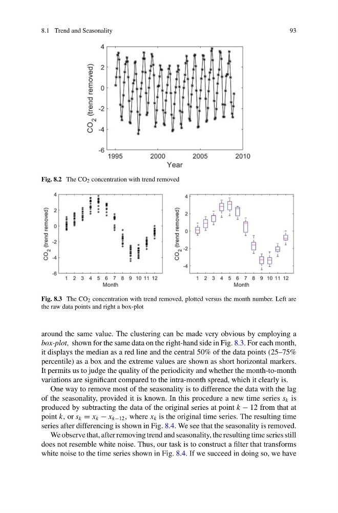
Fig. 8.2 The CO 2 concentration with trend removed
Fig. 8.3 The CO 2 concentration with trend removed, plotted versus the month number. Left are
the raw data points and right a box-plot
around the same value. The clustering can be made very obvious by employing a
box-plot, shown for the same data on the right-hand side in Fig. 8.3. For each month,
it displays the median as a red line and the central 50% of the data points (25–75%
percentile) as a box and the extreme values are shown as short horizontal markers.
It permits us to judge the quality of the periodicity and whether the month-to-month
variations are significant compared to the intra-month spread, which it clearly is.
One way to remove most of the seasonality is to difference the data with the lag
of the seasonality, provided it is known. In this procedure a new time series s k is
produced by subtracting the data of the original series at point k − 12 from that at
point k, or s k = x k − x k−12 , where x k is the original time series. The resulting time
series after differencing is shown in Fig. 8.4. We see that the seasonality is removed.
We observe that, after removing trend and seasonality, the resulting time series still
does not resemble white noise. Thus, our task is to construct a filter that transforms
white noise to the time series shown in Fig. 8.4. If we succeed in doing so, we have
93
Fig. 8.2 The CO 2 concentration with trend removed
Fig. 8.3 The CO 2 concentration with trend removed, plotted versus the month number. Left are
the raw data points and right a box-plot
around the same value. The clustering can be made very obvious by employing a
box-plot, shown for the same data on the right-hand side in Fig. 8.3. For each month,
it displays the median as a red line and the central 50% of the data points (25–75%
percentile) as a box and the extreme values are shown as short horizontal markers.
It permits us to judge the quality of the periodicity and whether the month-to-month
variations are significant compared to the intra-month spread, which it clearly is.
One way to remove most of the seasonality is to difference the data with the lag
of the seasonality, provided it is known. In this procedure a new time series s k is
produced by subtracting the data of the original series at point k − 12 from that at
point k, or s k = x k − x k−12 , where x k is the original time series. The resulting time
series after differencing is shown in Fig. 8.4. We see that the seasonality is removed.
We observe that, after removing trend and seasonality, the resulting time series still
does not resemble white noise. Thus, our task is to construct a filter that transforms
white noise to the time series shown in Fig. 8.4. If we succeed in doing so, we have