

92
8 Time Series
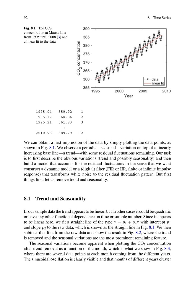
Fig. 8.1 The CO 2
concentration at Mauna Loa
from 1995 until 2008 [3] and
a linear fit to the data
1995.04
359.92
1
1995.12
360.86
2
1995.21
361.83
3
:
2010.96
389.79
12
We can obtain a first impression of the data by simply plotting the data points, as
shown in Fig. 8.1. We observe a periodic—seasonal—variation on top of a linearly
increasing base line—a trend—with some residual fluctuations remaining. Our task
is to first describe the obvious variations (trend and possibly seasonality) and then
build a model that accounts for the residual fluctuations in the sense that we want
construct a dynamic model or a (digital) filter (FIR or IIR, finite or infinite impulse
response) that transforms white noise to the residual fluctuation pattern. But first
things first: let us remove trend and seasonality.
8.1 Trend and Seasonality
In our sample data the trend appears to be linear, but in other cases it could be quadratic
or have any other functional dependence on time or sample number. Since it appears
to be linear here, we fit a straight line of the type y = p 1 + p 2 x with intercept p 1
and slope p 2 to the raw data, which is shown as the straight line in Fig. 8.1. We then
subtract that line from the raw data and show the result in Fig. 8.2, where the trend
is removed and the seasonal variations are the most prominent remaining feature.
The seasonal variations become apparent when plotting the CO 2 concentration
after trend removal as a function of the month, which is what we show in Fig. 8.3,
where there are several data points at each month coming from the different years.
The sinusoidal oscillation is clearly visible and that months of different years cluster
8 Time Series
Fig. 8.1 The CO 2
concentration at Mauna Loa
from 1995 until 2008 [3] and
a linear fit to the data
1995.04
359.92
1
1995.12
360.86
2
1995.21
361.83
3
:
2010.96
389.79
12
We can obtain a first impression of the data by simply plotting the data points, as
shown in Fig. 8.1. We observe a periodic—seasonal—variation on top of a linearly
increasing base line—a trend—with some residual fluctuations remaining. Our task
is to first describe the obvious variations (trend and possibly seasonality) and then
build a model that accounts for the residual fluctuations in the sense that we want
construct a dynamic model or a (digital) filter (FIR or IIR, finite or infinite impulse
response) that transforms white noise to the residual fluctuation pattern. But first
things first: let us remove trend and seasonality.
8.1 Trend and Seasonality
In our sample data the trend appears to be linear, but in other cases it could be quadratic
or have any other functional dependence on time or sample number. Since it appears
to be linear here, we fit a straight line of the type y = p 1 + p 2 x with intercept p 1
and slope p 2 to the raw data, which is shown as the straight line in Fig. 8.1. We then
subtract that line from the raw data and show the result in Fig. 8.2, where the trend
is removed and the seasonal variations are the most prominent remaining feature.
The seasonal variations become apparent when plotting the CO 2 concentration
after trend removal as a function of the month, which is what we show in Fig. 8.3,
where there are several data points at each month coming from the different years.
The sinusoidal oscillation is clearly visible and that months of different years cluster