

94
8 Time Series
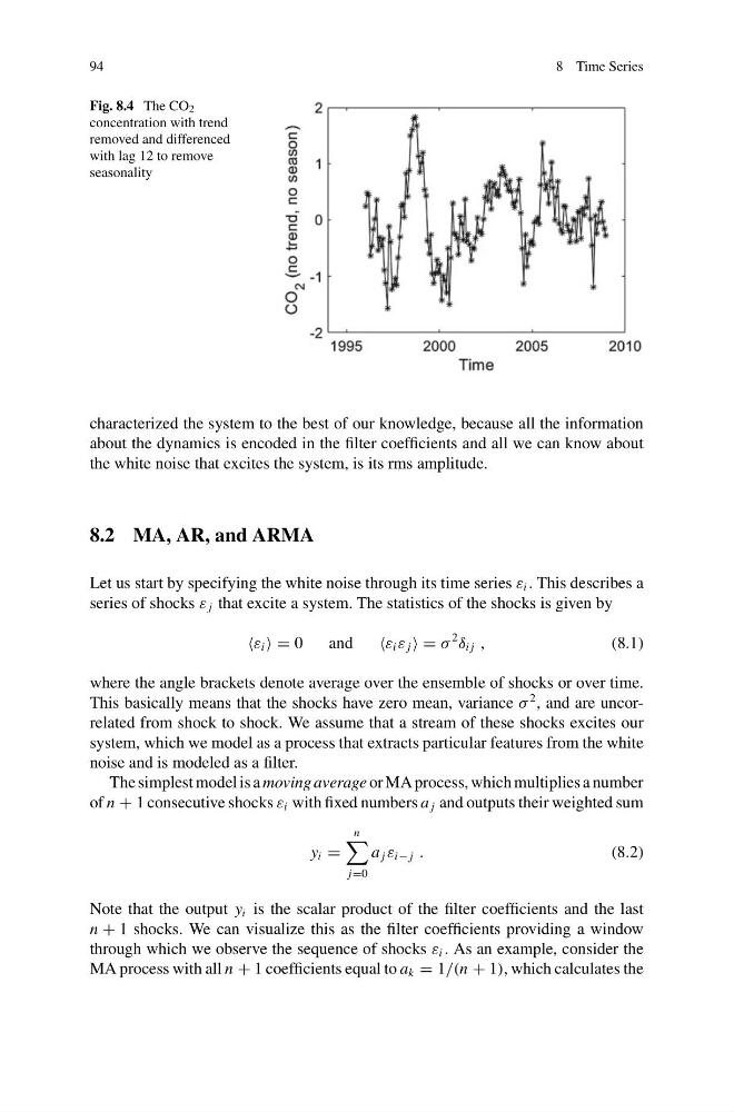
Fig. 8.4 The CO 2
concentration with trend
removed and differenced
with lag 12 to remove
seasonality
characterized the system to the best of our knowledge, because all the information
about the dynamics is encoded in the filter coefficients and all we can know about
the white noise that excites the system, is its rms amplitude.
8.2 MA, AR, and ARMA
Let us start by specifying the white noise through its time series ε i . This describes a
series of shocks ε j that excite a system. The statistics of the shocks is given by
ε i = 0
and
ε i ε j = σ
2
δ i j ,
(8.1)
where the angle brackets denote average over the ensemble of shocks or over time.
This basically means that the shocks have zero mean, variance σ
2 , and are uncorrelated from shock to shock. We assume that a stream of these shocks excites our
system, which we model as a process that extracts particular features from the white
noise and is modeled as a filter.
The simplest model is a moving average or MA process, which multiplies a number
of n + 1 consecutive shocks ε i with fixed numbers a j and outputs their weighted sum
y i =
n
j=0
a j ε i− j .
(8.2)
Note that the output y i is the scalar product of the filter coefficients and the last
n + 1 shocks. We can visualize this as the filter coefficients providing a window
through which we observe the sequence of shocks ε i . As an example, consider the
MA process with all n + 1 coefficients equal to a k = 1/(n + 1), which calculates the
8 Time Series
Fig. 8.4 The CO 2
concentration with trend
removed and differenced
with lag 12 to remove
seasonality
characterized the system to the best of our knowledge, because all the information
about the dynamics is encoded in the filter coefficients and all we can know about
the white noise that excites the system, is its rms amplitude.
8.2 MA, AR, and ARMA
Let us start by specifying the white noise through its time series ε i . This describes a
series of shocks ε j that excite a system. The statistics of the shocks is given by
ε i = 0
and
ε i ε j = σ
2
δ i j ,
(8.1)
where the angle brackets denote average over the ensemble of shocks or over time.
This basically means that the shocks have zero mean, variance σ
2 , and are uncorrelated from shock to shock. We assume that a stream of these shocks excites our
system, which we model as a process that extracts particular features from the white
noise and is modeled as a filter.
The simplest model is a moving average or MA process, which multiplies a number
of n + 1 consecutive shocks ε i with fixed numbers a j and outputs their weighted sum
y i =
n
j=0
a j ε i− j .
(8.2)
Note that the output y i is the scalar product of the filter coefficients and the last
n + 1 shocks. We can visualize this as the filter coefficients providing a window
through which we observe the sequence of shocks ε i . As an example, consider the
MA process with all n + 1 coefficients equal to a k = 1/(n + 1), which calculates the