

406
11 Nonlinear Dynamics of Circuits with Mem-Elements
with state variables q λ (t; t 0 ) (we let ϕ λ
0 = L λ i
γ
0 ).
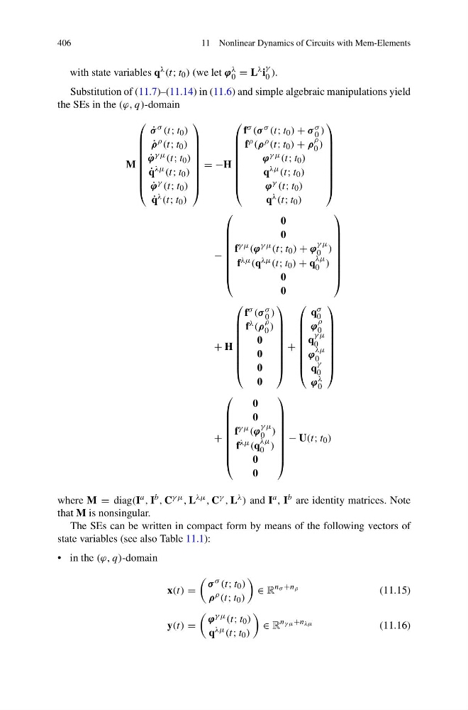
Substitution of (11.7)–(11.14) in (11.6) and simple algebraic manipulations yield
the SEs in the (ϕ, q)-domain
M
⎛
⎜
⎜
⎜
⎜
⎜
⎜
⎜
⎝
˙
σ σ (t; t 0 )
˙
ρ ρ (t; t 0 )
˙
ϕ γ μ (t; t 0 )
˙
q λμ (t; t 0 )
˙
ϕ γ (t; t 0 )
˙
q λ (t; t 0 )
⎞
⎟
⎟
⎟
⎟
⎟
⎟
⎟
⎠
= −H
⎛
⎜
⎜
⎜
⎜
⎜
⎜
⎜
⎝
f σ (σ σ (t; t 0 ) + σ σ
0 )
f ρ (ρ ρ (t; t 0 ) + ρ
ρ
0 )
ϕ γ μ (t; t 0 )
q λμ (t; t 0 )
ϕ γ (t; t 0 )
q λ (t; t 0 )
⎞
⎟
⎟
⎟
⎟
⎟
⎟
⎟
⎠
−
⎛
⎜
⎜
⎜
⎜
⎜
⎜
⎜
⎝
0
0
f γ μ (ϕ γ μ (t; t 0 ) + ϕ
γ μ
0 )
f λμ (q λμ (t; t 0 ) + q
λμ
0 )
0
0
⎞
⎟
⎟
⎟
⎟
⎟
⎟
⎟
⎠
+ H
⎛
⎜
⎜
⎜
⎜
⎜
⎜
⎜
⎝
f σ (σ σ
0 )
f λ (ρ
ρ
0 )
0
0
0
0
⎞
⎟
⎟
⎟
⎟
⎟
⎟
⎟
⎠
+
⎛
⎜
⎜
⎜
⎜
⎜
⎜
⎜
⎝
q σ
0
ϕ
ρ
0
q
γ μ
0
ϕ
λμ
0
q
γ
0
ϕ λ
0
⎞
⎟
⎟
⎟
⎟
⎟
⎟
⎟
⎠
+
⎛
⎜
⎜
⎜
⎜
⎜
⎜
⎜
⎝
0
0
f γ μ (ϕ
γ μ
0 )
f λμ (q
λμ
0 )
0
0
⎞
⎟
⎟
⎟
⎟
⎟
⎟
⎟
⎠
− U(t; t 0 )
where M = diag(I a , I b , C γ μ , L λμ , C γ , L λ ) and I a , I b are identity matrices. Note
that M is nonsingular.
The SEs can be written in compact form by means of the following vectors of
state variables (see also Table 11.1):
• in the (ϕ, q)-domain
x(t) =
σ σ (t; t 0 )
ρ ρ (t; t 0 )
∈ R
n σ +n ρ
(11.15)
y(t) =
ϕ γ μ (t; t 0 )
q λμ (t; t 0 )
∈ R
n γ μ +n λμ
(11.16)
11 Nonlinear Dynamics of Circuits with Mem-Elements
with state variables q λ (t; t 0 ) (we let ϕ λ
0 = L λ i
γ
0 ).
Substitution of (11.7)–(11.14) in (11.6) and simple algebraic manipulations yield
the SEs in the (ϕ, q)-domain
M
⎛
⎜
⎜
⎜
⎜
⎜
⎜
⎜
⎝
˙
σ σ (t; t 0 )
˙
ρ ρ (t; t 0 )
˙
ϕ γ μ (t; t 0 )
˙
q λμ (t; t 0 )
˙
ϕ γ (t; t 0 )
˙
q λ (t; t 0 )
⎞
⎟
⎟
⎟
⎟
⎟
⎟
⎟
⎠
= −H
⎛
⎜
⎜
⎜
⎜
⎜
⎜
⎜
⎝
f σ (σ σ (t; t 0 ) + σ σ
0 )
f ρ (ρ ρ (t; t 0 ) + ρ
ρ
0 )
ϕ γ μ (t; t 0 )
q λμ (t; t 0 )
ϕ γ (t; t 0 )
q λ (t; t 0 )
⎞
⎟
⎟
⎟
⎟
⎟
⎟
⎟
⎠
−
⎛
⎜
⎜
⎜
⎜
⎜
⎜
⎜
⎝
0
0
f γ μ (ϕ γ μ (t; t 0 ) + ϕ
γ μ
0 )
f λμ (q λμ (t; t 0 ) + q
λμ
0 )
0
0
⎞
⎟
⎟
⎟
⎟
⎟
⎟
⎟
⎠
+ H
⎛
⎜
⎜
⎜
⎜
⎜
⎜
⎜
⎝
f σ (σ σ
0 )
f λ (ρ
ρ
0 )
0
0
0
0
⎞
⎟
⎟
⎟
⎟
⎟
⎟
⎟
⎠
+
⎛
⎜
⎜
⎜
⎜
⎜
⎜
⎜
⎝
q σ
0
ϕ
ρ
0
q
γ μ
0
ϕ
λμ
0
q
γ
0
ϕ λ
0
⎞
⎟
⎟
⎟
⎟
⎟
⎟
⎟
⎠
+
⎛
⎜
⎜
⎜
⎜
⎜
⎜
⎜
⎝
0
0
f γ μ (ϕ
γ μ
0 )
f λμ (q
λμ
0 )
0
0
⎞
⎟
⎟
⎟
⎟
⎟
⎟
⎟
⎠
− U(t; t 0 )
where M = diag(I a , I b , C γ μ , L λμ , C γ , L λ ) and I a , I b are identity matrices. Note
that M is nonsingular.
The SEs can be written in compact form by means of the following vectors of
state variables (see also Table 11.1):
• in the (ϕ, q)-domain
x(t) =
σ σ (t; t 0 )
ρ ρ (t; t 0 )
∈ R
n σ +n ρ
(11.15)
y(t) =
ϕ γ μ (t; t 0 )
q λμ (t; t 0 )
∈ R
n γ μ +n λμ
(11.16)