

404
11 Nonlinear Dynamics of Circuits with Mem-Elements
Table 11.1 State variables and O
(α,β)
D
(v, i)-domain
(ϕ, q)-domain
D
State variables
O
(0,0)
D
ICs
State variables O
(−1,−1)
D
ICs RO
R (lin.)
–
0
–
–
0
–
0
e
–
0
–
–
0
–
0
a
–
0
–
–
0
–
0
C (lin.)
v C (t)
1
v C 0
ϕ C (t; t 0 )
1
0
0
L (lin.)
i L (t)
1
i L 0
q L (t; t 0 )
1
0
0
C q (nonlin.) q C (t)
1
q C 0
ϕ C (t; t 0 )
1
0
0
L ϕ (nonlin.) ϕ L (t)
1
ϕ L 0
q L (t; t 0 )
1
0
0
M ϕ
ϕ M (t)
1
ϕ M 0
–
0
–
1
M q
q M (t)
1
q M 0
–
0
–
1
MC σ
σ MC (t), q MC (t) 2
σ MC 0 , q MC 0 σ MC (t; t 0 )
1
0
1
ML ρ
ρ ML (t), ϕ ML (t) 2
ρ ML 0 , ϕ ML 0 ρ ML (t; t 0 )
1
0
1
11.5 State Equations and Nonlinear Dynamics
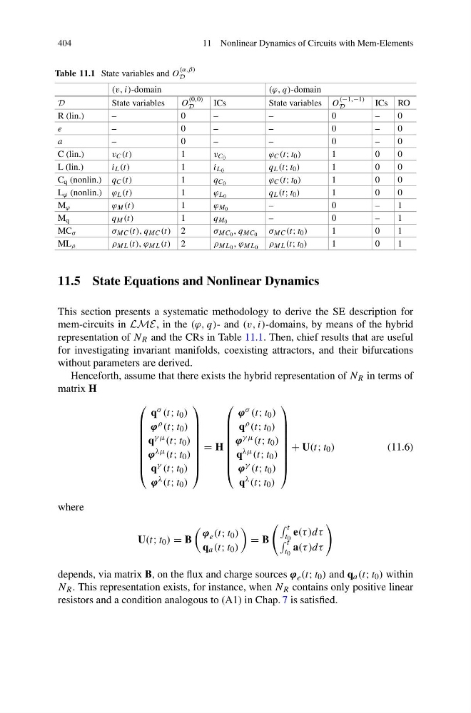
This section presents a systematic methodology to derive the SE description for
mem-circuits in LME, in the (ϕ, q)- and (v, i)-domains, by means of the hybrid
representation of N R and the CRs in Table 11.1. Then, chief results that are useful
for investigating invariant manifolds, coexisting attractors, and their bifurcations
without parameters are derived.
Henceforth, assume that there exists the hybrid representation of N R in terms of
matrix H
⎛
⎜
⎜
⎜
⎜
⎜
⎜
⎜
⎝
q σ (t; t 0 )
ϕ ρ (t; t 0 )
q γ μ (t; t 0 )
ϕ λμ (t; t 0 )
q γ (t; t 0 )
ϕ λ (t; t 0 )
⎞
⎟
⎟
⎟
⎟
⎟
⎟
⎟
⎠
= H
⎛
⎜
⎜
⎜
⎜
⎜
⎜
⎜
⎝
ϕ σ (t; t 0 )
q ρ (t; t 0 )
ϕ γ μ (t; t 0 )
q λμ (t; t 0 )
ϕ γ (t; t 0 )
q λ (t; t 0 )
⎞
⎟
⎟
⎟
⎟
⎟
⎟
⎟
⎠
+ U(t; t 0 )
(11.6)
where
U(t; t 0 ) = B
ϕ e (t; t 0 )
q a (t; t 0 )
= B
t
t 0
e(τ )dτ
t
t 0
a(τ )dτ
depends, via matrix B, on the flux and charge sources ϕ e (t; t 0 ) and q a (t; t 0 ) within
N R . This representation exists, for instance, when N R contains only positive linear
resistors and a condition analogous to (A1) in Chap. 7 is satisfied.
11 Nonlinear Dynamics of Circuits with Mem-Elements
Table 11.1 State variables and O
(α,β)
D
(v, i)-domain
(ϕ, q)-domain
D
State variables
O
(0,0)
D
ICs
State variables O
(−1,−1)
D
ICs RO
R (lin.)
–
0
–
–
0
–
0
e
–
0
–
–
0
–
0
a
–
0
–
–
0
–
0
C (lin.)
v C (t)
1
v C 0
ϕ C (t; t 0 )
1
0
0
L (lin.)
i L (t)
1
i L 0
q L (t; t 0 )
1
0
0
C q (nonlin.) q C (t)
1
q C 0
ϕ C (t; t 0 )
1
0
0
L ϕ (nonlin.) ϕ L (t)
1
ϕ L 0
q L (t; t 0 )
1
0
0
M ϕ
ϕ M (t)
1
ϕ M 0
–
0
–
1
M q
q M (t)
1
q M 0
–
0
–
1
MC σ
σ MC (t), q MC (t) 2
σ MC 0 , q MC 0 σ MC (t; t 0 )
1
0
1
ML ρ
ρ ML (t), ϕ ML (t) 2
ρ ML 0 , ϕ ML 0 ρ ML (t; t 0 )
1
0
1
11.5 State Equations and Nonlinear Dynamics
This section presents a systematic methodology to derive the SE description for
mem-circuits in LME, in the (ϕ, q)- and (v, i)-domains, by means of the hybrid
representation of N R and the CRs in Table 11.1. Then, chief results that are useful
for investigating invariant manifolds, coexisting attractors, and their bifurcations
without parameters are derived.
Henceforth, assume that there exists the hybrid representation of N R in terms of
matrix H
⎛
⎜
⎜
⎜
⎜
⎜
⎜
⎜
⎝
q σ (t; t 0 )
ϕ ρ (t; t 0 )
q γ μ (t; t 0 )
ϕ λμ (t; t 0 )
q γ (t; t 0 )
ϕ λ (t; t 0 )
⎞
⎟
⎟
⎟
⎟
⎟
⎟
⎟
⎠
= H
⎛
⎜
⎜
⎜
⎜
⎜
⎜
⎜
⎝
ϕ σ (t; t 0 )
q ρ (t; t 0 )
ϕ γ μ (t; t 0 )
q λμ (t; t 0 )
ϕ γ (t; t 0 )
q λ (t; t 0 )
⎞
⎟
⎟
⎟
⎟
⎟
⎟
⎟
⎠
+ U(t; t 0 )
(11.6)
where
U(t; t 0 ) = B
ϕ e (t; t 0 )
q a (t; t 0 )
= B
t
t 0
e(τ )dτ
t
t 0
a(τ )dτ
depends, via matrix B, on the flux and charge sources ϕ e (t; t 0 ) and q a (t; t 0 ) within
N R . This representation exists, for instance, when N R contains only positive linear
resistors and a condition analogous to (A1) in Chap. 7 is satisfied.