

288
7 Pulse Programming of Memristor Circuits
• M and G are diagonal matrices defined as
M = diag(C γ M , L λ M , C γ G , L λ R , C γ C , L λ L )
and
G = diag(0, 0, G γ G , R λ R , 0, 0).
In particular, we have the following:
• M is nonsingular;
• the state variables in the (ϕ, q)-domain are the n C fluxes across the capacitors
(i.e., ϕ γ M (t; t 0 ), ϕ γ G (t; t 0 ) and ϕ γ C (t; t 0 )) and n L charges through the inductors
(i.e., q λ M (t; t 0 ), q λ R (t; t 0 ) and q λ L (t; t 0 )); the ICs at t 0 are by construction null;
• (7.16) is a system of n = n C + n L SEs where the first n M = γ M + λ M equations
are nonlinear, whereas the other (n C + n L − n M ) equations are linear;
• since N R is linear, vector u(t, t 0 ) in (7.12) can be explicitly written in terms of
the internal sources as
u(t; t 0 ) = B
ϕ e (t; t 0 )
q a (t; t 0 )
with B ∈ R (n C +n L )×(n E +n A ) . 5
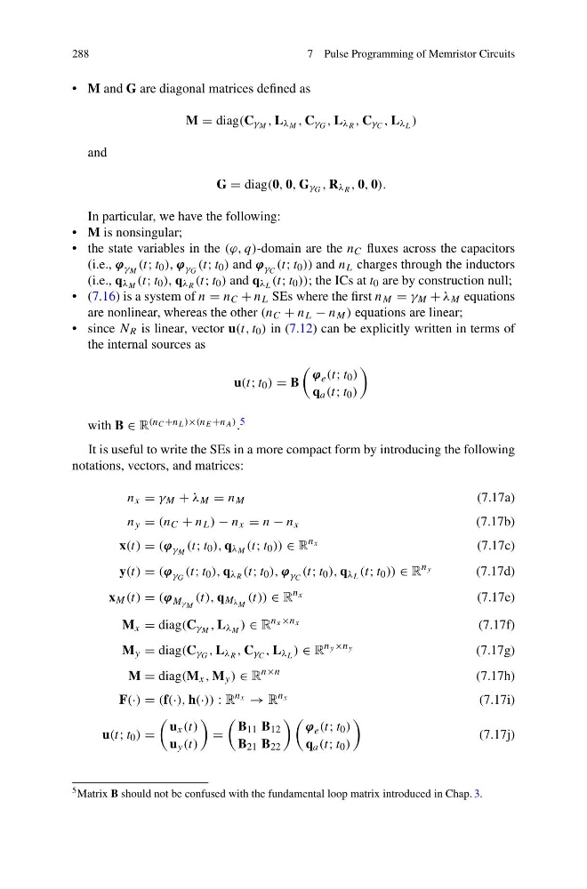
It is useful to write the SEs in a more compact form by introducing the following
notations, vectors, and matrices:
n x = γ M + λ M = n M
(7.17a)
n y = (n C + n L ) − n x = n − n x
(7.17b)
x(t) = (ϕ γ M (t; t 0 ), q λ M (t; t 0 )) ∈ R
n x
(7.17c)
y(t) = (ϕ γ G (t; t 0 ), q λ R (t; t 0 ), ϕ γ C (t; t 0 ), q λ L (t; t 0 )) ∈ R
n y
(7.17d)
x M (t) = (ϕ M γ M
(t), q M λ M (t)) ∈ R
n x
(7.17e)
M x = diag(C γ M , L λ M ) ∈ R
n x ×n x
(7.17f)
M y = diag(C γ G , L λ R , C γ C , L λ L ) ∈ R
n y ×n y
(7.17g)
M = diag(M x , M y ) ∈ R
n×n
(7.17h)
F(·) = (f(·), h(·)) : R
n x → R
n x
(7.17i)
u(t; t 0 ) =
u x (t)
u y (t)
=
B 11 B 12
B 21 B 22
ϕ e (t; t 0 )
q a (t; t 0 )
(7.17j)
5 Matrix B should not be confused with the fundamental loop matrix introduced in Chap. 3.
7 Pulse Programming of Memristor Circuits
• M and G are diagonal matrices defined as
M = diag(C γ M , L λ M , C γ G , L λ R , C γ C , L λ L )
and
G = diag(0, 0, G γ G , R λ R , 0, 0).
In particular, we have the following:
• M is nonsingular;
• the state variables in the (ϕ, q)-domain are the n C fluxes across the capacitors
(i.e., ϕ γ M (t; t 0 ), ϕ γ G (t; t 0 ) and ϕ γ C (t; t 0 )) and n L charges through the inductors
(i.e., q λ M (t; t 0 ), q λ R (t; t 0 ) and q λ L (t; t 0 )); the ICs at t 0 are by construction null;
• (7.16) is a system of n = n C + n L SEs where the first n M = γ M + λ M equations
are nonlinear, whereas the other (n C + n L − n M ) equations are linear;
• since N R is linear, vector u(t, t 0 ) in (7.12) can be explicitly written in terms of
the internal sources as
u(t; t 0 ) = B
ϕ e (t; t 0 )
q a (t; t 0 )
with B ∈ R (n C +n L )×(n E +n A ) . 5
It is useful to write the SEs in a more compact form by introducing the following
notations, vectors, and matrices:
n x = γ M + λ M = n M
(7.17a)
n y = (n C + n L ) − n x = n − n x
(7.17b)
x(t) = (ϕ γ M (t; t 0 ), q λ M (t; t 0 )) ∈ R
n x
(7.17c)
y(t) = (ϕ γ G (t; t 0 ), q λ R (t; t 0 ), ϕ γ C (t; t 0 ), q λ L (t; t 0 )) ∈ R
n y
(7.17d)
x M (t) = (ϕ M γ M
(t), q M λ M (t)) ∈ R
n x
(7.17e)
M x = diag(C γ M , L λ M ) ∈ R
n x ×n x
(7.17f)
M y = diag(C γ G , L λ R , C γ C , L λ L ) ∈ R
n y ×n y
(7.17g)
M = diag(M x , M y ) ∈ R
n×n
(7.17h)
F(·) = (f(·), h(·)) : R
n x → R
n x
(7.17i)
u(t; t 0 ) =
u x (t)
u y (t)
=
B 11 B 12
B 21 B 22
ϕ e (t; t 0 )
q a (t; t 0 )
(7.17j)
5 Matrix B should not be confused with the fundamental loop matrix introduced in Chap. 3.