

7.4 State Equations in the Flux-Charge Domain
289
H = H R + G =
H 11 H 12
H 21 H 22
(7.17k)
where H 11 ∈ R n x ×n x , H 12 ∈ R n x ×n y , H 21 ∈ R n y ×n x , and H 22 ∈ R n y ×n y , whereas
B 11 ∈ R n x ×n E , B 12 ∈ R n x ×n A , B 21 ∈ R n y ×n E , and B 22 ∈ R n y ×n A .
Note that x M (t) is the vector of fluxes and charges in the memristors and we have
x M (t) = x(t) + x M (t 0 ) ⇒ ˙
x M (t) = ˙
x(t), ∀t ≥ t 0 .
(7.18)
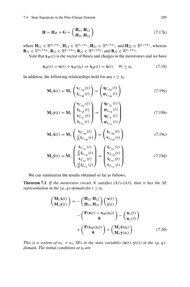
In addition, the following relationships hold for any t ≥ t 0 :
M x ˙
x(t) = M x
v C γ M (t)
i L λ M (t)
=
q C γ M (t)
ϕ L λ M
(t)
(7.19a)
M y ˙
y(t) = M y
⎛
⎜
⎜
⎜
⎝
v C γ G (t)
i L λ R (t)
v C γ C (t)
i L λ L (t)
⎞
⎟
⎟
⎟
⎠
=
⎛
⎜
⎜
⎜
⎝
q C γ G (t)
ϕ L λ R
(t)
q C γ C (t)
ϕ L λ L
(t)
⎞
⎟
⎟
⎟
⎠
(7.19b)
M x ¨
x(t) = M x
˙
v C γ M (t)
d
dt i L λ M (t)
=
i C γ M (t)
v L λ M (t)
(7.19c)
M y ¨
y(t) = M y
⎛
⎜
⎜
⎜
⎝
˙
v C γ G (t)
d
dt i L λ R (t)
˙
v C γ C (t)
d
dt i L λ L (t)
⎞
⎟
⎟
⎟
⎠
=
⎛
⎜
⎜
⎜
⎝
i C γ G (t)
v L λ R (t)
i C γ C (t)
v L λ L (t)
⎞
⎟
⎟
⎟
⎠
.
(7.19d)
We can summarize the results obtained so far as follows.
Theorem 7.1 If the memristor circuit N satisfies (A1)–(A3), then it has the SE
representation in the (ϕ, q)-domain for t ≥ t 0
M x ˙
x(t)
M y ˙
y(t)
= −
H 11 H 12
H 21 H 22
x(t)
y(t)
−
F(x(t) + x M (t 0 ))
0
−
u x (t)
u y (t)
+
F(x M (t 0 ))
0
+
M x ˙
x(t 0 )
M y ˙
y(t 0 )
.
(7.20)
This is a system of n C + n L SEs in the state variables (x(t), y(t)) in the (ϕ, q)domain. The initial conditions at t 0 are
289
H = H R + G =
H 11 H 12
H 21 H 22
(7.17k)
where H 11 ∈ R n x ×n x , H 12 ∈ R n x ×n y , H 21 ∈ R n y ×n x , and H 22 ∈ R n y ×n y , whereas
B 11 ∈ R n x ×n E , B 12 ∈ R n x ×n A , B 21 ∈ R n y ×n E , and B 22 ∈ R n y ×n A .
Note that x M (t) is the vector of fluxes and charges in the memristors and we have
x M (t) = x(t) + x M (t 0 ) ⇒ ˙
x M (t) = ˙
x(t), ∀t ≥ t 0 .
(7.18)
In addition, the following relationships hold for any t ≥ t 0 :
M x ˙
x(t) = M x
v C γ M (t)
i L λ M (t)
=
q C γ M (t)
ϕ L λ M
(t)
(7.19a)
M y ˙
y(t) = M y
⎛
⎜
⎜
⎜
⎝
v C γ G (t)
i L λ R (t)
v C γ C (t)
i L λ L (t)
⎞
⎟
⎟
⎟
⎠
=
⎛
⎜
⎜
⎜
⎝
q C γ G (t)
ϕ L λ R
(t)
q C γ C (t)
ϕ L λ L
(t)
⎞
⎟
⎟
⎟
⎠
(7.19b)
M x ¨
x(t) = M x
˙
v C γ M (t)
d
dt i L λ M (t)
=
i C γ M (t)
v L λ M (t)
(7.19c)
M y ¨
y(t) = M y
⎛
⎜
⎜
⎜
⎝
˙
v C γ G (t)
d
dt i L λ R (t)
˙
v C γ C (t)
d
dt i L λ L (t)
⎞
⎟
⎟
⎟
⎠
=
⎛
⎜
⎜
⎜
⎝
i C γ G (t)
v L λ R (t)
i C γ C (t)
v L λ L (t)
⎞
⎟
⎟
⎟
⎠
.
(7.19d)
We can summarize the results obtained so far as follows.
Theorem 7.1 If the memristor circuit N satisfies (A1)–(A3), then it has the SE
representation in the (ϕ, q)-domain for t ≥ t 0
M x ˙
x(t)
M y ˙
y(t)
= −
H 11 H 12
H 21 H 22
x(t)
y(t)
−
F(x(t) + x M (t 0 ))
0
−
u x (t)
u y (t)
+
F(x M (t 0 ))
0
+
M x ˙
x(t 0 )
M y ˙
y(t 0 )
.
(7.20)
This is a system of n C + n L SEs in the state variables (x(t), y(t)) in the (ϕ, q)domain. The initial conditions at t 0 are