

256
6 Memristor Circuits: Invariant Manifolds, Coexisting Attractors, Extreme. . .
n(x(t)) = Rf (x(t)) = −Rax + Rbx
3
= −m 0 x(t) + m 1 x(t)
3 .
(6.41)
Moreover,
X 0 =
β
β + γ
ϕ M 0 +
β
β + γ
Li L 0 +
γ
β + γ
RC 2 v C 2 0 + n(ϕ M 0 ) + RC 1 v C 1 0
(6.42)
which is a term depending on the initial conditions for the state variables
v C 1 0 , v C 2 0 , i L 0 , and ϕ M 0 of the MCC in the (v, i)-domain.
Remark 6.21 It is stressed that (6.40) with X 0 = 0 describes the dynamics of the
well-known canonical Chua’s oscillator (Chap. 4). Instead, when X 0 = 0, (6.40)
describes the dynamics of a Chua’s oscillator with a constant forcing term. Again,
this enables to use the bulk of results for Chua’s oscillator in the analysis of MCC
in the (ϕ, q)-domain.
Invariant Manifolds
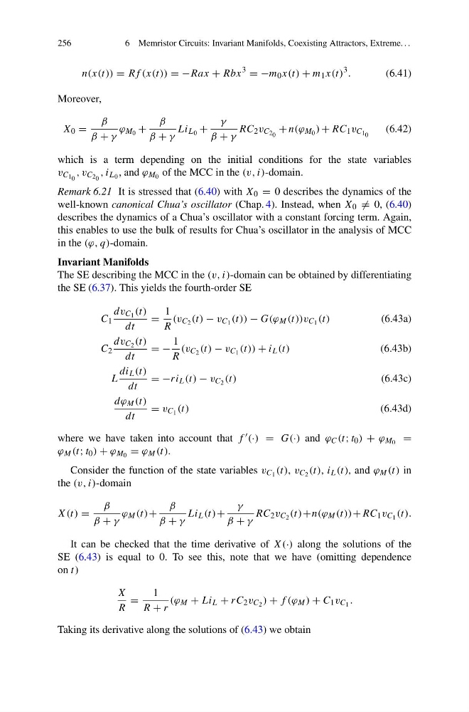
The SE describing the MCC in the (v, i)-domain can be obtained by differentiating
the SE (6.37). This yields the fourth-order SE
C 1
dv C 1 (t)
dt
=
1
R
(v C 2 (t) − v C 1 (t)) − G(ϕ M (t))v C 1 (t)
(6.43a)
C 2
dv C 2 (t)
dt
= −
1
R
(v C 2 (t) − v C 1 (t)) + i L (t)
(6.43b)
L
di L (t)
dt
= −ri L (t) − v C 2 (t)
(6.43c)
dϕ M (t)
dt
= v C 1 (t)
(6.43d)
where we have taken into account that f (·) = G(·) and ϕ C (t; t 0 ) + ϕ M 0 =
ϕ M (t; t 0 ) + ϕ M 0 = ϕ M (t).
Consider the function of the state variables v C 1 (t), v C 2 (t), i L (t), and ϕ M (t) in
the (v, i)-domain
X(t) =
β
β + γ
ϕ M (t)+
β
β + γ
Li L (t)+
γ
β + γ
RC 2 v C 2 (t)+n(ϕ M (t))+RC 1 v C 1 (t).
It can be checked that the time derivative of X(·) along the solutions of the
SE (6.43) is equal to 0. To see this, note that we have (omitting dependence
on t)
X
R
=
1
R + r
(ϕ M + Li L + rC 2 v C 2 ) + f (ϕ M ) + C 1 v C 1 .
Taking its derivative along the solutions of (6.43) we obtain
6 Memristor Circuits: Invariant Manifolds, Coexisting Attractors, Extreme. . .
n(x(t)) = Rf (x(t)) = −Rax + Rbx
3
= −m 0 x(t) + m 1 x(t)
3 .
(6.41)
Moreover,
X 0 =
β
β + γ
ϕ M 0 +
β
β + γ
Li L 0 +
γ
β + γ
RC 2 v C 2 0 + n(ϕ M 0 ) + RC 1 v C 1 0
(6.42)
which is a term depending on the initial conditions for the state variables
v C 1 0 , v C 2 0 , i L 0 , and ϕ M 0 of the MCC in the (v, i)-domain.
Remark 6.21 It is stressed that (6.40) with X 0 = 0 describes the dynamics of the
well-known canonical Chua’s oscillator (Chap. 4). Instead, when X 0 = 0, (6.40)
describes the dynamics of a Chua’s oscillator with a constant forcing term. Again,
this enables to use the bulk of results for Chua’s oscillator in the analysis of MCC
in the (ϕ, q)-domain.
Invariant Manifolds
The SE describing the MCC in the (v, i)-domain can be obtained by differentiating
the SE (6.37). This yields the fourth-order SE
C 1
dv C 1 (t)
dt
=
1
R
(v C 2 (t) − v C 1 (t)) − G(ϕ M (t))v C 1 (t)
(6.43a)
C 2
dv C 2 (t)
dt
= −
1
R
(v C 2 (t) − v C 1 (t)) + i L (t)
(6.43b)
L
di L (t)
dt
= −ri L (t) − v C 2 (t)
(6.43c)
dϕ M (t)
dt
= v C 1 (t)
(6.43d)
where we have taken into account that f (·) = G(·) and ϕ C (t; t 0 ) + ϕ M 0 =
ϕ M (t; t 0 ) + ϕ M 0 = ϕ M (t).
Consider the function of the state variables v C 1 (t), v C 2 (t), i L (t), and ϕ M (t) in
the (v, i)-domain
X(t) =
β
β + γ
ϕ M (t)+
β
β + γ
Li L (t)+
γ
β + γ
RC 2 v C 2 (t)+n(ϕ M (t))+RC 1 v C 1 (t).
It can be checked that the time derivative of X(·) along the solutions of the
SE (6.43) is equal to 0. To see this, note that we have (omitting dependence
on t)
X
R
=
1
R + r
(ϕ M + Li L + rC 2 v C 2 ) + f (ϕ M ) + C 1 v C 1 .
Taking its derivative along the solutions of (6.43) we obtain