

6.2 Second-Order Memristor Oscillators
249
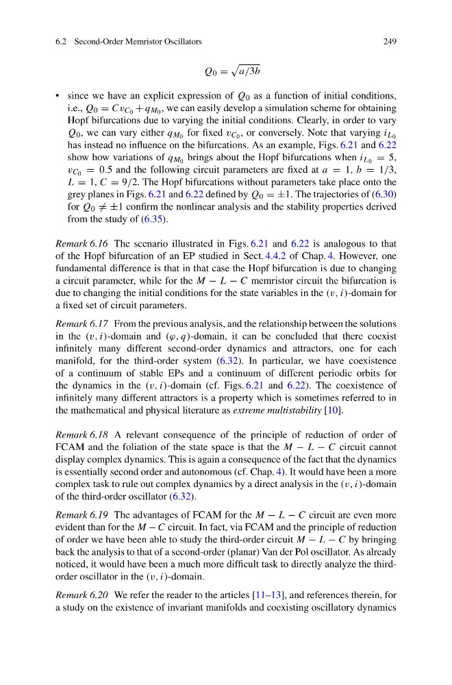
Q 0 =
a/3b
• since we have an explicit expression of Q 0 as a function of initial conditions,
i.e., Q 0 = Cv C 0 + q M 0 , we can easily develop a simulation scheme for obtaining
Hopf bifurcations due to varying the initial conditions. Clearly, in order to vary
Q 0 , we can vary either q M 0 for fixed v C 0 , or conversely. Note that varying i L 0
has instead no influence on the bifurcations. As an example, Figs. 6.21 and 6.22
show how variations of q M 0 brings about the Hopf bifurcations when i L 0 = 5,
v C 0 = 0.5 and the following circuit parameters are fixed at a = 1, b = 1/3,
L = 1, C = 9/2. The Hopf bifurcations without parameters take place onto the
grey planes in Figs. 6.21 and 6.22 defined by Q 0 = ±1. The trajectories of (6.30)
for Q 0 = ±1 confirm the nonlinear analysis and the stability properties derived
from the study of (6.35).
Remark 6.16 The scenario illustrated in Figs. 6.21 and 6.22 is analogous to that
of the Hopf bifurcation of an EP studied in Sect. 4.4.2 of Chap. 4. However, one
fundamental difference is that in that case the Hopf bifurcation is due to changing
a circuit parameter, while for the M − L − C memristor circuit the bifurcation is
due to changing the initial conditions for the state variables in the (v, i)-domain for
a fixed set of circuit parameters.
Remark 6.17 From the previous analysis, and the relationship between the solutions
in the (v, i)-domain and (ϕ, q)-domain, it can be concluded that there coexist
infinitely many different second-order dynamics and attractors, one for each
manifold, for the third-order system (6.32). In particular, we have coexistence
of a continuum of stable EPs and a continuum of different periodic orbits for
the dynamics in the (v, i)-domain (cf. Figs. 6.21 and 6.22). The coexistence of
infinitely many different attractors is a property which is sometimes referred to in
the mathematical and physical literature as extreme multistability [10].
Remark 6.18 A relevant consequence of the principle of reduction of order of
FCAM and the foliation of the state space is that the M − L − C circuit cannot
display complex dynamics. This is again a consequence of the fact that the dynamics
is essentially second order and autonomous (cf. Chap. 4). It would have been a more
complex task to rule out complex dynamics by a direct analysis in the (v, i)-domain
of the third-order oscillator (6.32).
Remark 6.19 The advantages of FCAM for the M − L − C circuit are even more
evident than for the M − C circuit. In fact, via FCAM and the principle of reduction
of order we have been able to study the third-order circuit M − L − C by bringing
back the analysis to that of a second-order (planar) Van der Pol oscillator. As already
noticed, it would have been a much more difficult task to directly analyze the thirdorder oscillator in the (v, i)-domain.
Remark 6.20 We refer the reader to the articles [11–13], and references therein, for
a study on the existence of invariant manifolds and coexisting oscillatory dynamics
249
Q 0 =
a/3b
• since we have an explicit expression of Q 0 as a function of initial conditions,
i.e., Q 0 = Cv C 0 + q M 0 , we can easily develop a simulation scheme for obtaining
Hopf bifurcations due to varying the initial conditions. Clearly, in order to vary
Q 0 , we can vary either q M 0 for fixed v C 0 , or conversely. Note that varying i L 0
has instead no influence on the bifurcations. As an example, Figs. 6.21 and 6.22
show how variations of q M 0 brings about the Hopf bifurcations when i L 0 = 5,
v C 0 = 0.5 and the following circuit parameters are fixed at a = 1, b = 1/3,
L = 1, C = 9/2. The Hopf bifurcations without parameters take place onto the
grey planes in Figs. 6.21 and 6.22 defined by Q 0 = ±1. The trajectories of (6.30)
for Q 0 = ±1 confirm the nonlinear analysis and the stability properties derived
from the study of (6.35).
Remark 6.16 The scenario illustrated in Figs. 6.21 and 6.22 is analogous to that
of the Hopf bifurcation of an EP studied in Sect. 4.4.2 of Chap. 4. However, one
fundamental difference is that in that case the Hopf bifurcation is due to changing
a circuit parameter, while for the M − L − C memristor circuit the bifurcation is
due to changing the initial conditions for the state variables in the (v, i)-domain for
a fixed set of circuit parameters.
Remark 6.17 From the previous analysis, and the relationship between the solutions
in the (v, i)-domain and (ϕ, q)-domain, it can be concluded that there coexist
infinitely many different second-order dynamics and attractors, one for each
manifold, for the third-order system (6.32). In particular, we have coexistence
of a continuum of stable EPs and a continuum of different periodic orbits for
the dynamics in the (v, i)-domain (cf. Figs. 6.21 and 6.22). The coexistence of
infinitely many different attractors is a property which is sometimes referred to in
the mathematical and physical literature as extreme multistability [10].
Remark 6.18 A relevant consequence of the principle of reduction of order of
FCAM and the foliation of the state space is that the M − L − C circuit cannot
display complex dynamics. This is again a consequence of the fact that the dynamics
is essentially second order and autonomous (cf. Chap. 4). It would have been a more
complex task to rule out complex dynamics by a direct analysis in the (v, i)-domain
of the third-order oscillator (6.32).
Remark 6.19 The advantages of FCAM for the M − L − C circuit are even more
evident than for the M − C circuit. In fact, via FCAM and the principle of reduction
of order we have been able to study the third-order circuit M − L − C by bringing
back the analysis to that of a second-order (planar) Van der Pol oscillator. As already
noticed, it would have been a much more difficult task to directly analyze the thirdorder oscillator in the (v, i)-domain.
Remark 6.20 We refer the reader to the articles [11–13], and references therein, for
a study on the existence of invariant manifolds and coexisting oscillatory dynamics