

5.8 Formulation of Memristor Circuits Equations
215
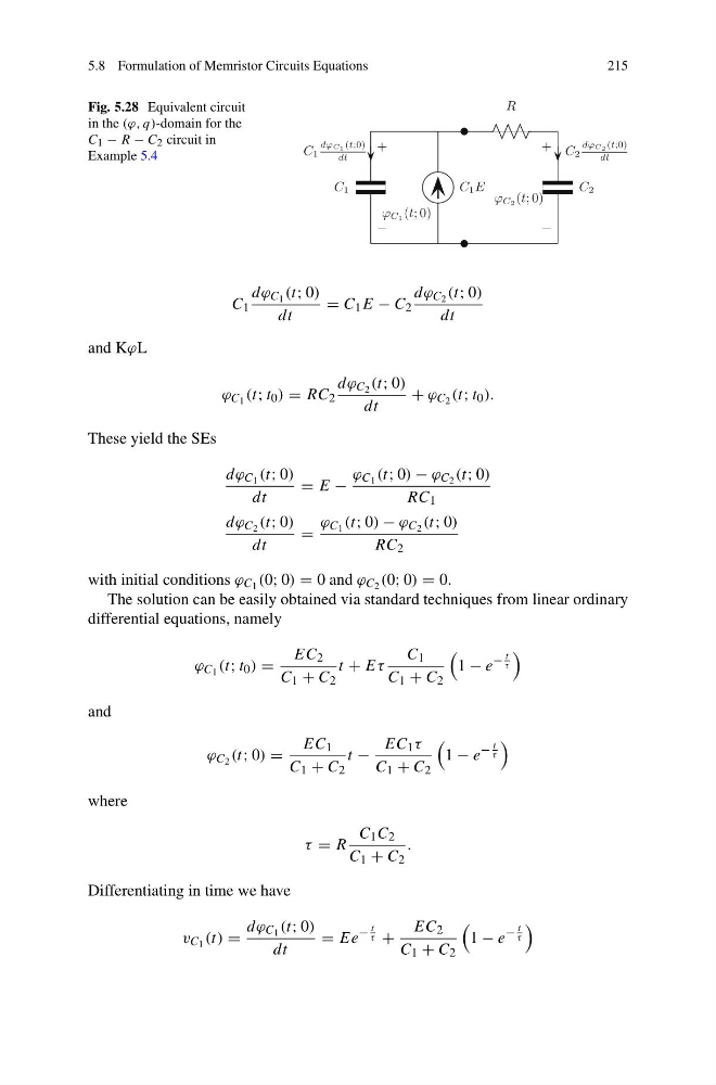
Fig. 5.28 Equivalent circuit
in the (ϕ, q)-domain for the
C 1 − R − C 2 circuit in
Example 5.4
C 1
dϕ C 1 (t; 0)
dt
= C 1 E − C 2
dϕ C 2 (t; 0)
dt
and KϕL
ϕ C 1 (t; t 0 ) = RC 2
dϕ C 2 (t; 0)
dt
+ ϕ C 2 (t; t 0 ).
These yield the SEs
dϕ C 1 (t; 0)
dt
= E −
ϕ C 1 (t; 0) − ϕ C 2 (t; 0)
RC 1
dϕ C 2 (t; 0)
dt
=
ϕ C 1 (t; 0) − ϕ C 2 (t; 0)
RC 2
with initial conditions ϕ C 1 (0; 0) = 0 and ϕ C 2 (0; 0) = 0.
The solution can be easily obtained via standard techniques from linear ordinary
differential equations, namely
ϕ C 1 (t; t 0 ) =
EC 2
C 1 + C 2
t + Eτ
C 1
C 1 + C 2
1 − e
−
t
τ
and
ϕ C 2 (t; 0) =
EC 1
C 1 + C 2
t −
EC 1 τ
C 1 + C 2
1 − e
−
t
τ
where
τ = R
C 1 C 2
C 1 + C 2
.
Differentiating in time we have
v C 1 (t) =
dϕ C 1 (t; 0)
dt
= Ee
−
t
τ +
EC 2
C 1 + C 2
1 − e
−
t
τ
215
Fig. 5.28 Equivalent circuit
in the (ϕ, q)-domain for the
C 1 − R − C 2 circuit in
Example 5.4
C 1
dϕ C 1 (t; 0)
dt
= C 1 E − C 2
dϕ C 2 (t; 0)
dt
and KϕL
ϕ C 1 (t; t 0 ) = RC 2
dϕ C 2 (t; 0)
dt
+ ϕ C 2 (t; t 0 ).
These yield the SEs
dϕ C 1 (t; 0)
dt
= E −
ϕ C 1 (t; 0) − ϕ C 2 (t; 0)
RC 1
dϕ C 2 (t; 0)
dt
=
ϕ C 1 (t; 0) − ϕ C 2 (t; 0)
RC 2
with initial conditions ϕ C 1 (0; 0) = 0 and ϕ C 2 (0; 0) = 0.
The solution can be easily obtained via standard techniques from linear ordinary
differential equations, namely
ϕ C 1 (t; t 0 ) =
EC 2
C 1 + C 2
t + Eτ
C 1
C 1 + C 2
1 − e
−
t
τ
and
ϕ C 2 (t; 0) =
EC 1
C 1 + C 2
t −
EC 1 τ
C 1 + C 2
1 − e
−
t
τ
where
τ = R
C 1 C 2
C 1 + C 2
.
Differentiating in time we have
v C 1 (t) =
dϕ C 1 (t; 0)
dt
= Ee
−
t
τ +
EC 2
C 1 + C 2
1 − e
−
t
τ