

5.3 Fundamental Examples on Kirchhoff Laws
173
q C 1 (t; 0) + q C 2 (t; 0) = 0
for any t ≥ 0. This yields
q C 1 (t; 0) + q C 2 (t; 0) = C 1 v C 1 (t) − C 1 v C 1 (0) + C 2 v C 2 (t) − C 2 v C 2 (0) = 0
hence
q C 1 (t) + q C 2 (t) = C 1 v C 1 (0) = C 1 E
for t ≥ 0, which is indeed the correct equation describing the conservation of charge
for t ≥ 0. Note that here we used only the information on the initial conditions
v C 1 (0) = E and v C 2 (0) = 0.
For the moment we stop here with the analysis in the (ϕ, q)-domain of this
circuit, since the current goal is to illustrate the difficulties in using the first
form (5.3) of conservation of charge. Later in the chapter, after developing the fluxcharge analysis method, we will come back to this circuit and complete its analysis
in the (ϕ, q)-domain (see Example 5.20).
Example 5.5 Consider again the sub-circuit C 1 -R-C 2 as in Fig. 5.2 of Example 5.4
for t ≥ t 0 = 0. Let v C 1 (0) = 0, v C 2 (0) = 0. Suppose such initial conditions are
available from measurements at t = 0 but we do not know the history of the circuit
for t ≤ 0, i.e., we do not know how the initial conditions are created for t ≤ 0. As
already discussed, the charge conservation law in the form q C 1 (t) + q C 2 (t) = 0 for
t ≥ 0 is not valid. Since the information on the history of the circuit for t ≤ 0 is
not available, we are forced to use the third form of conservation of charge, i.e., the
incremental form
q C 1 (t; 0) + q C 2 (t; 0) = 0
which involves only the behavior of the circuit for t ≥ 0. Note that this is all we
need to arrive at the correct result q C 1 (t) + q C 2 (t) = C 1 v C 1 (0) for t ≥ 0.
Example 5.6 This example aims at highlighting difficulties in using the second
form given in (5.5) and (5.6) of Kirchhoff laws in the (ϕ, q)-domain.
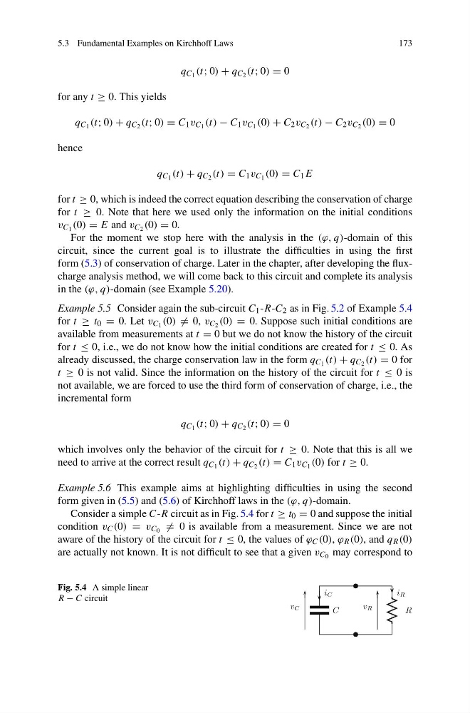
Consider a simple C-R circuit as in Fig. 5.4 for t ≥ t 0 = 0 and suppose the initial
condition v C (0) = v C 0 = 0 is available from a measurement. Since we are not
aware of the history of the circuit for t ≤ 0, the values of ϕ C (0), ϕ R (0), and q R (0)
are actually not known. It is not difficult to see that a given v C 0 may correspond to
Fig. 5.4 A simple linear
R − C circuit
173
q C 1 (t; 0) + q C 2 (t; 0) = 0
for any t ≥ 0. This yields
q C 1 (t; 0) + q C 2 (t; 0) = C 1 v C 1 (t) − C 1 v C 1 (0) + C 2 v C 2 (t) − C 2 v C 2 (0) = 0
hence
q C 1 (t) + q C 2 (t) = C 1 v C 1 (0) = C 1 E
for t ≥ 0, which is indeed the correct equation describing the conservation of charge
for t ≥ 0. Note that here we used only the information on the initial conditions
v C 1 (0) = E and v C 2 (0) = 0.
For the moment we stop here with the analysis in the (ϕ, q)-domain of this
circuit, since the current goal is to illustrate the difficulties in using the first
form (5.3) of conservation of charge. Later in the chapter, after developing the fluxcharge analysis method, we will come back to this circuit and complete its analysis
in the (ϕ, q)-domain (see Example 5.20).
Example 5.5 Consider again the sub-circuit C 1 -R-C 2 as in Fig. 5.2 of Example 5.4
for t ≥ t 0 = 0. Let v C 1 (0) = 0, v C 2 (0) = 0. Suppose such initial conditions are
available from measurements at t = 0 but we do not know the history of the circuit
for t ≤ 0, i.e., we do not know how the initial conditions are created for t ≤ 0. As
already discussed, the charge conservation law in the form q C 1 (t) + q C 2 (t) = 0 for
t ≥ 0 is not valid. Since the information on the history of the circuit for t ≤ 0 is
not available, we are forced to use the third form of conservation of charge, i.e., the
incremental form
q C 1 (t; 0) + q C 2 (t; 0) = 0
which involves only the behavior of the circuit for t ≥ 0. Note that this is all we
need to arrive at the correct result q C 1 (t) + q C 2 (t) = C 1 v C 1 (0) for t ≥ 0.
Example 5.6 This example aims at highlighting difficulties in using the second
form given in (5.5) and (5.6) of Kirchhoff laws in the (ϕ, q)-domain.
Consider a simple C-R circuit as in Fig. 5.4 for t ≥ t 0 = 0 and suppose the initial
condition v C (0) = v C 0 = 0 is available from a measurement. Since we are not
aware of the history of the circuit for t ≤ 0, the values of ϕ C (0), ϕ R (0), and q R (0)
are actually not known. It is not difficult to see that a given v C 0 may correspond to
Fig. 5.4 A simple linear
R − C circuit