

134
4 Nonlinear Dynamics and Bifurcations in Autonomous RLC Circuits
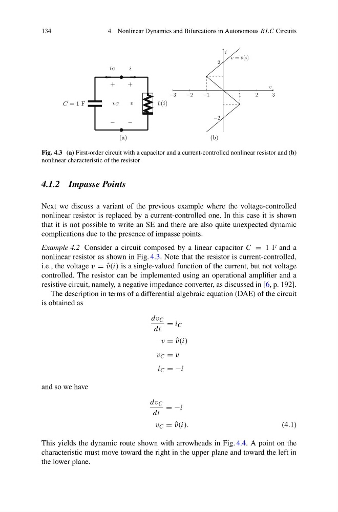
Fig. 4.3 (a) First-order circuit with a capacitor and a current-controlled nonlinear resistor and (b)
nonlinear characteristic of the resistor
4.1.2 Impasse Points
Next we discuss a variant of the previous example where the voltage-controlled
nonlinear resistor is replaced by a current-controlled one. In this case it is shown
that it is not possible to write an SE and there are also quite unexpected dynamic
complications due to the presence of impasse points.
Example 4.2 Consider a circuit composed by a linear capacitor C = 1 F and a
nonlinear resistor as shown in Fig. 4.3. Note that the resistor is current-controlled,
i.e., the voltage v = ˆ
v(i) is a single-valued function of the current, but not voltage
controlled. The resistor can be implemented using an operational amplifier and a
resistive circuit, namely, a negative impedance converter, as discussed in [6, p. 192].
The description in terms of a differential algebraic equation (DAE) of the circuit
is obtained as
dv C
dt
= i C
v = ˆ
v(i)
v C = v
i C = −i
and so we have
dv C
dt
= −i
v C = ˆ
v(i).
(4.1)
This yields the dynamic route shown with arrowheads in Fig. 4.4. A point on the
characteristic must move toward the right in the upper plane and toward the left in
the lower plane.
4 Nonlinear Dynamics and Bifurcations in Autonomous RLC Circuits
Fig. 4.3 (a) First-order circuit with a capacitor and a current-controlled nonlinear resistor and (b)
nonlinear characteristic of the resistor
4.1.2 Impasse Points
Next we discuss a variant of the previous example where the voltage-controlled
nonlinear resistor is replaced by a current-controlled one. In this case it is shown
that it is not possible to write an SE and there are also quite unexpected dynamic
complications due to the presence of impasse points.
Example 4.2 Consider a circuit composed by a linear capacitor C = 1 F and a
nonlinear resistor as shown in Fig. 4.3. Note that the resistor is current-controlled,
i.e., the voltage v = ˆ
v(i) is a single-valued function of the current, but not voltage
controlled. The resistor can be implemented using an operational amplifier and a
resistive circuit, namely, a negative impedance converter, as discussed in [6, p. 192].
The description in terms of a differential algebraic equation (DAE) of the circuit
is obtained as
dv C
dt
= i C
v = ˆ
v(i)
v C = v
i C = −i
and so we have
dv C
dt
= −i
v C = ˆ
v(i).
(4.1)
This yields the dynamic route shown with arrowheads in Fig. 4.4. A point on the
characteristic must move toward the right in the upper plane and toward the left in
the lower plane.