

3.2 Tableau Analysis
111
Thus, the set of 12 linear algebraic equations (3.14), (3.17), and (3.33) in the 12
unknowns v k and i k (k = 1, 2, . . . , 6) permit to describe and solve the circuit in
Fig. 3.4.
Remark 3.3 Introducing the vectors of branch currents i = (i t , i l ) T and voltages
v = (v t , v l ) T organized in terms of twig and link variables of the tree T 3 in Fig. 3.2c,
i.e.,
i t = (i 2 , i 4 , i 5 )
T
v t = (v 2 , v 4 , v 5 )
T
i l = (i 1 , i 3 , i 6 )
T
v l = (v 1 , v 3 , v 6 )
T
the cut-set tableau equations can be written in the compact form
Qi = 0
(3.34)
v = Q
T v t
(3.35)
i = Gv − a
(3.36)
where (3.36) represents the matrix form of (3.33). Matrix G is a 6 × 6 diagonal
matrix including the conductances of resistors, i.e., G = diag(G 2 , G 4 , G 5 , 0, G 3 , G 6 )
and a = (0, 0, 0, a 1 , 0, 0) T . Simple algebraic manipulations permit to reduce the
cut-set tableau equations to
QGQ
T v t = Q
T a
(3.37)
which includes just three equations. It is important to observe that if a tree T is
picked in such a way that Q coincides with A, then (3.37) describes the nodal
analysis method. Further details on the nodal analysis (and the dual mesh analysis)
can be found in [1].
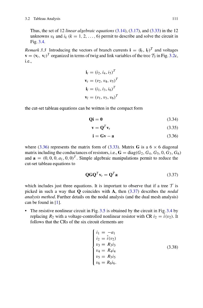
• The resistive nonlinear circuit in Fig. 3.5 is obtained by the circuit in Fig. 3.4 by
replacing R 2 with a voltage-controlled nonlinear resistor with CR i 2 = ˆ
i(v 2 ). It
follows that the CRs of the six circuit elements are
⎧
⎪ ⎪ ⎪ ⎪ ⎪ ⎪ ⎪ ⎨
⎪ ⎪ ⎪ ⎪ ⎪ ⎪ ⎪ ⎩
i 1 = −a 1
i 2 = ˆ
i(v 2 )
v 3 = R 3 i 3
v 4 = R 4 i 4
v 5 = R 5 i 5
v 6 = R 6 i 6 .
(3.38)
111
Thus, the set of 12 linear algebraic equations (3.14), (3.17), and (3.33) in the 12
unknowns v k and i k (k = 1, 2, . . . , 6) permit to describe and solve the circuit in
Fig. 3.4.
Remark 3.3 Introducing the vectors of branch currents i = (i t , i l ) T and voltages
v = (v t , v l ) T organized in terms of twig and link variables of the tree T 3 in Fig. 3.2c,
i.e.,
i t = (i 2 , i 4 , i 5 )
T
v t = (v 2 , v 4 , v 5 )
T
i l = (i 1 , i 3 , i 6 )
T
v l = (v 1 , v 3 , v 6 )
T
the cut-set tableau equations can be written in the compact form
Qi = 0
(3.34)
v = Q
T v t
(3.35)
i = Gv − a
(3.36)
where (3.36) represents the matrix form of (3.33). Matrix G is a 6 × 6 diagonal
matrix including the conductances of resistors, i.e., G = diag(G 2 , G 4 , G 5 , 0, G 3 , G 6 )
and a = (0, 0, 0, a 1 , 0, 0) T . Simple algebraic manipulations permit to reduce the
cut-set tableau equations to
QGQ
T v t = Q
T a
(3.37)
which includes just three equations. It is important to observe that if a tree T is
picked in such a way that Q coincides with A, then (3.37) describes the nodal
analysis method. Further details on the nodal analysis (and the dual mesh analysis)
can be found in [1].
• The resistive nonlinear circuit in Fig. 3.5 is obtained by the circuit in Fig. 3.4 by
replacing R 2 with a voltage-controlled nonlinear resistor with CR i 2 = ˆ
i(v 2 ). It
follows that the CRs of the six circuit elements are
⎧
⎪ ⎪ ⎪ ⎪ ⎪ ⎪ ⎪ ⎨
⎪ ⎪ ⎪ ⎪ ⎪ ⎪ ⎪ ⎩
i 1 = −a 1
i 2 = ˆ
i(v 2 )
v 3 = R 3 i 3
v 4 = R 4 i 4
v 5 = R 5 i 5
v 6 = R 6 i 6 .
(3.38)