

110
3 RLC Networks Equations and Analysis Methods
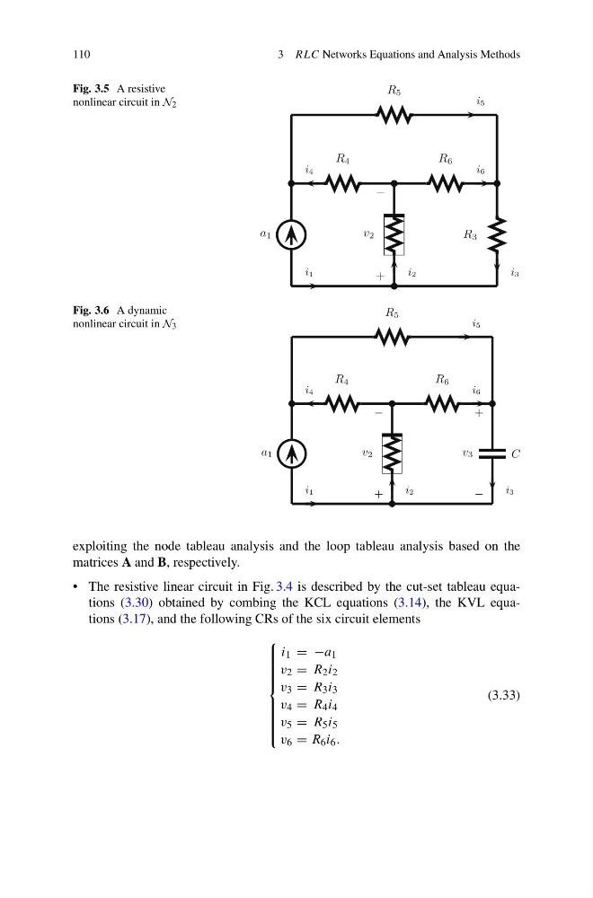
Fig. 3.5 A resistive
nonlinear circuit in N 2
a 1
R 5
R 4
R 6
v 2
R 3
i1
i2
i3
i4
i6
i5
+
−
Fig. 3.6 A dynamic
nonlinear circuit in N 3
a 1
R 5
R 4
R 6
v 2
C
v 3
i1
i2
i3
i4
i6
i5
+
−
−
+
exploiting the node tableau analysis and the loop tableau analysis based on the
matrices A and B, respectively.
• The resistive linear circuit in Fig. 3.4 is described by the cut-set tableau equations (3.30) obtained by combing the KCL equations (3.14), the KVL equations (3.17), and the following CRs of the six circuit elements
⎧
⎪ ⎪ ⎪ ⎪ ⎪ ⎪ ⎪ ⎨
⎪ ⎪ ⎪ ⎪ ⎪ ⎪ ⎪ ⎩
i 1 = −a 1
v 2 = R 2 i 2
v 3 = R 3 i 3
v 4 = R 4 i 4
v 5 = R 5 i 5
v 6 = R 6 i 6 .
(3.33)
3 RLC Networks Equations and Analysis Methods
Fig. 3.5 A resistive
nonlinear circuit in N 2
a 1
R 5
R 4
R 6
v 2
R 3
i1
i2
i3
i4
i6
i5
+
−
Fig. 3.6 A dynamic
nonlinear circuit in N 3
a 1
R 5
R 4
R 6
v 2
C
v 3
i1
i2
i3
i4
i6
i5
+
−
−
+
exploiting the node tableau analysis and the loop tableau analysis based on the
matrices A and B, respectively.
• The resistive linear circuit in Fig. 3.4 is described by the cut-set tableau equations (3.30) obtained by combing the KCL equations (3.14), the KVL equations (3.17), and the following CRs of the six circuit elements
⎧
⎪ ⎪ ⎪ ⎪ ⎪ ⎪ ⎪ ⎨
⎪ ⎪ ⎪ ⎪ ⎪ ⎪ ⎪ ⎩
i 1 = −a 1
v 2 = R 2 i 2
v 3 = R 3 i 3
v 4 = R 4 i 4
v 5 = R 5 i 5
v 6 = R 6 i 6 .
(3.33)