

3.2 Tableau Analysis
109
⎧
⎨
⎩
Bv = 0
i = B T i l
f(v (α) , i (β) ) = 0
(3.32)
where v (α) = (v
(α 1 )
1 , v
(α 2 )
2 , . . . , v
(α b )
b ) T , i (β) = (i
(β 1 )
1 , i
(β 2 )
2 , . . . , i
(β b )
b ) T , and f =
(f 1 , f 2 , . . . , f b ) T : R 2b → R b .
Remark 3.2 Whenever possible, it is convenient from a mathematical viewpoint
to avoid the use of integral equations, i.e., to write the tableau equations avoiding
α k , β k < 0. This yields via the tableau a system of differential algebraic equations
(DAEs).
Example 3.4 (Cut-Set Tableau Analysis) Let us consider a class of networks N with
topology as in Fig. 3.1a and described by the digraph in Fig. 3.1b. Different classes
of networks can be specified according to the properties of the two-terminal circuit
elements in N . In this example the cut-set tableau analysis is presented for the
following classes:
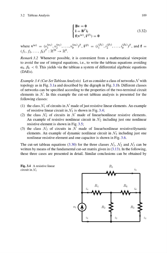
(1) the class N 1 of circuits in N made of just resistive linear elements. An example
of resistive linear circuit in N 1 is shown in Fig. 3.4;
(2) the class N 2 of circuits in N made of linear/nonlinear resistive elements.
An example of resistive nonlinear circuit in N 2 including just one nonlinear
resistive element is shown in Fig. 3.5;
(3) the class N 3 of circuits in N made of linear/nonlinear resistive/dynamic
elements. An example of dynamic nonlinear circuit in N 3 including just one
nonlinear resistive element and one capacitor is shown in Fig. 3.6.
The cut-set tableau equations (3.30) for the three classes N 1 , N 2 and N 3 can be
written by means of the fundamental cut-set matrix given in (3.13). In the following,
these three cases are presented in detail. Similar conclusions can be obtained by
Fig. 3.4 A resistive linear
circuit in N 1
a 1
R 5
R 4
R 6
R 2
R 3
i1
i2
i3
i4
i6
i5
109
⎧
⎨
⎩
Bv = 0
i = B T i l
f(v (α) , i (β) ) = 0
(3.32)
where v (α) = (v
(α 1 )
1 , v
(α 2 )
2 , . . . , v
(α b )
b ) T , i (β) = (i
(β 1 )
1 , i
(β 2 )
2 , . . . , i
(β b )
b ) T , and f =
(f 1 , f 2 , . . . , f b ) T : R 2b → R b .
Remark 3.2 Whenever possible, it is convenient from a mathematical viewpoint
to avoid the use of integral equations, i.e., to write the tableau equations avoiding
α k , β k < 0. This yields via the tableau a system of differential algebraic equations
(DAEs).
Example 3.4 (Cut-Set Tableau Analysis) Let us consider a class of networks N with
topology as in Fig. 3.1a and described by the digraph in Fig. 3.1b. Different classes
of networks can be specified according to the properties of the two-terminal circuit
elements in N . In this example the cut-set tableau analysis is presented for the
following classes:
(1) the class N 1 of circuits in N made of just resistive linear elements. An example
of resistive linear circuit in N 1 is shown in Fig. 3.4;
(2) the class N 2 of circuits in N made of linear/nonlinear resistive elements.
An example of resistive nonlinear circuit in N 2 including just one nonlinear
resistive element is shown in Fig. 3.5;
(3) the class N 3 of circuits in N made of linear/nonlinear resistive/dynamic
elements. An example of dynamic nonlinear circuit in N 3 including just one
nonlinear resistive element and one capacitor is shown in Fig. 3.6.
The cut-set tableau equations (3.30) for the three classes N 1 , N 2 and N 3 can be
written by means of the fundamental cut-set matrix given in (3.13). In the following,
these three cases are presented in detail. Similar conclusions can be obtained by
Fig. 3.4 A resistive linear
circuit in N 1
a 1
R 5
R 4
R 6
R 2
R 3
i1
i2
i3
i4
i6
i5