

3.7 Active Suspensions
61
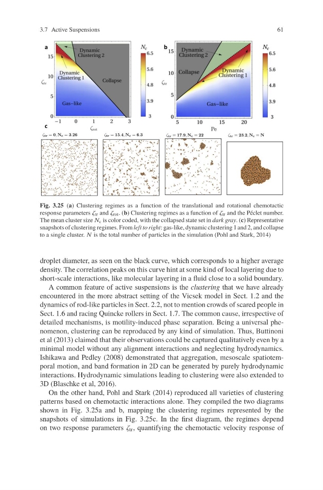
Fig. 3.25 (a) Clustering regimes as a function of the translational and rotational chemotactic
response parameters ζ tr and ζ rot . (b) Clustering regimes as a function of ζ tr and the Péclet number.
The mean cluster size N c is color coded, with the collapsed state set in dark gray. (c) Representative
snapshots of clustering regimes. From left to right: gas-like, dynamic clustering 1 and 2, and collapse
to a single cluster. N is the total number of particles in the simulation (Pohl and Stark, 2014)
droplet diameter, as seen on the black curve, which corresponds to a higher average
density. The correlation peaks on this curve hint at some kind of local layering due to
short-scale interactions, like molecular layering in a fluid close to a solid boundary.
A common feature of active suspensions is the clustering that we have already
encountered in the more abstract setting of the Vicsek model in Sect. 1.2 and the
dynamics of rod-like particles in Sect. 2.2, not to mention crowds of scared people in
Sect. 1.6 and racing Quincke rollers in Sect. 1.7. The common cause, irrespective of
detailed mechanisms, is motility-induced phase separation. Being a universal phenomenon, clustering can be reproduced by any kind of simulation. Thus, Buttinoni
et al (2013) claimed that their observations could be captured qualitatively even by a
minimal model without any alignment interactions and neglecting hydrodynamics.
Ishikawa and Pedley (2008) demonstrated that aggregation, mesoscale spatiotemporal motion, and band formation in 2D can be generated by purely hydrodynamic
interactions. Hydrodynamic simulations leading to clustering were also extended to
3D (Blaschke et al, 2016).
On the other hand, Pohl and Stark (2014) reproduced all varieties of clustering
patterns based on chemotactic interactions alone. They compiled the two diagrams
shown in Fig. 3.25a and b, mapping the clustering regimes represented by the
snapshots of simulations in Fig. 3.25c. In the first diagram, the regimes depend
on two response parameters ζ tr , quantifying the chemotactic velocity response of
61
Fig. 3.25 (a) Clustering regimes as a function of the translational and rotational chemotactic
response parameters ζ tr and ζ rot . (b) Clustering regimes as a function of ζ tr and the Péclet number.
The mean cluster size N c is color coded, with the collapsed state set in dark gray. (c) Representative
snapshots of clustering regimes. From left to right: gas-like, dynamic clustering 1 and 2, and collapse
to a single cluster. N is the total number of particles in the simulation (Pohl and Stark, 2014)
droplet diameter, as seen on the black curve, which corresponds to a higher average
density. The correlation peaks on this curve hint at some kind of local layering due to
short-scale interactions, like molecular layering in a fluid close to a solid boundary.
A common feature of active suspensions is the clustering that we have already
encountered in the more abstract setting of the Vicsek model in Sect. 1.2 and the
dynamics of rod-like particles in Sect. 2.2, not to mention crowds of scared people in
Sect. 1.6 and racing Quincke rollers in Sect. 1.7. The common cause, irrespective of
detailed mechanisms, is motility-induced phase separation. Being a universal phenomenon, clustering can be reproduced by any kind of simulation. Thus, Buttinoni
et al (2013) claimed that their observations could be captured qualitatively even by a
minimal model without any alignment interactions and neglecting hydrodynamics.
Ishikawa and Pedley (2008) demonstrated that aggregation, mesoscale spatiotemporal motion, and band formation in 2D can be generated by purely hydrodynamic
interactions. Hydrodynamic simulations leading to clustering were also extended to
3D (Blaschke et al, 2016).
On the other hand, Pohl and Stark (2014) reproduced all varieties of clustering
patterns based on chemotactic interactions alone. They compiled the two diagrams
shown in Fig. 3.25a and b, mapping the clustering regimes represented by the
snapshots of simulations in Fig. 3.25c. In the first diagram, the regimes depend
on two response parameters ζ tr , quantifying the chemotactic velocity response of