

36
2 Active Nematics
2.6 Dynamics of Defects
The motion of defects determines to a large extent the flow pattern in active nematics.
One can see by comparing the two panels of Fig. 2.12 that the mean separation
between defects in the turbulent regime coincides with the typical vortex size. Defects
themselves permanently shift their positions due to induced flow, as well as by
inhomogeneities of nematic alignment that also depend on their locations. The
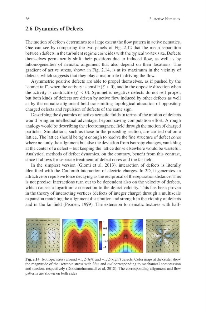
gradient of active stress, shown in Fig. 2.14, is at its maximum in the vicinity of
defects, which suggests that they play a major role in driving the flow.
Asymmetric positive defects are able to propel themselves, as if pushed by the
“comet tail”, when the activity is tensile (ζ > 0), and in the opposite direction when
the activity is contractile (ζ < 0). Symmetric negative defects do not self-propel,
but both kinds of defects are driven by active flow induced by other defects as well
as by the nematic alignment field transmitting topological attraction of oppositely
charged defects and repulsion of defects of the same sign.
Describing the dynamics of active nematic fluids in terms of the motion of defects
would bring an intellectual advantage, beyond saving computation effort. A rough
analogy would be describing the electromagnetic field through the motion of charged
particles. Simulations, such as those in the preceding section, are carried out on a
lattice. The lattice should be tight enough to resolve the fine structure of defect cores
where not only the alignment but also the deviation from isotropy changes, vanishing
at the center of a defect – but keeping the lattice dense elsewhere would be wasteful.
Analytical methods of defect dynamics, on the contrary, benefit from this contrast,
since it allows for separate treatment of defect cores and the far field.
In the simplest version (Giomi et al, 2013), interaction of defects is literally
identified with the Coulomb interaction of electric charges. In 2D, it generates an
attractive or repulsive force decaying as the reciprocal of the separation distance. This
is not precise: interactions turn out to be dependent also on the velocity of defects,
which causes a logarithmic correction to the defect velocity. This has been proven
in the theory of interacting vortices (defects of integer charge) through a multiscale
expansion matching the alignment distribution and strength in the vicinity of defects
and in the far field (Pismen, 1999). The extension to nematic textures with halfFig. 2.14 Isotropic stress around +1/2 (left) and −1/2 (right) defects. Color maps at the center show
the magnitude of the isotropic stress with blue and red corresponding to mechanical compression
and tension, respectively (Doostmohammadi et al, 2018). The corresponding alignment and flow
patterns are shown on both sides
2 Active Nematics
2.6 Dynamics of Defects
The motion of defects determines to a large extent the flow pattern in active nematics.
One can see by comparing the two panels of Fig. 2.12 that the mean separation
between defects in the turbulent regime coincides with the typical vortex size. Defects
themselves permanently shift their positions due to induced flow, as well as by
inhomogeneities of nematic alignment that also depend on their locations. The
gradient of active stress, shown in Fig. 2.14, is at its maximum in the vicinity of
defects, which suggests that they play a major role in driving the flow.
Asymmetric positive defects are able to propel themselves, as if pushed by the
“comet tail”, when the activity is tensile (ζ > 0), and in the opposite direction when
the activity is contractile (ζ < 0). Symmetric negative defects do not self-propel,
but both kinds of defects are driven by active flow induced by other defects as well
as by the nematic alignment field transmitting topological attraction of oppositely
charged defects and repulsion of defects of the same sign.
Describing the dynamics of active nematic fluids in terms of the motion of defects
would bring an intellectual advantage, beyond saving computation effort. A rough
analogy would be describing the electromagnetic field through the motion of charged
particles. Simulations, such as those in the preceding section, are carried out on a
lattice. The lattice should be tight enough to resolve the fine structure of defect cores
where not only the alignment but also the deviation from isotropy changes, vanishing
at the center of a defect – but keeping the lattice dense elsewhere would be wasteful.
Analytical methods of defect dynamics, on the contrary, benefit from this contrast,
since it allows for separate treatment of defect cores and the far field.
In the simplest version (Giomi et al, 2013), interaction of defects is literally
identified with the Coulomb interaction of electric charges. In 2D, it generates an
attractive or repulsive force decaying as the reciprocal of the separation distance. This
is not precise: interactions turn out to be dependent also on the velocity of defects,
which causes a logarithmic correction to the defect velocity. This has been proven
in the theory of interacting vortices (defects of integer charge) through a multiscale
expansion matching the alignment distribution and strength in the vicinity of defects
and in the far field (Pismen, 1999). The extension to nematic textures with halfFig. 2.14 Isotropic stress around +1/2 (left) and −1/2 (right) defects. Color maps at the center show
the magnitude of the isotropic stress with blue and red corresponding to mechanical compression
and tension, respectively (Doostmohammadi et al, 2018). The corresponding alignment and flow
patterns are shown on both sides